SlideShare a Scribd company logo
1 of 27
Download to read offline
UNIT - I
ELECTROSTATICS
Introduction
Charges at rest produce Static Electric Field or Electrostatic field.
Field: It is the existing space in particular area due to some elements.
1.1) Coulomb’s Law
Coulomb stated that the force between two point charges separated in a vacuum or free space
by a distance which is large compared to their size is
(i) proportional to the charge on each
(ii) inversely proportional to the square of the distance between them
(iii) directed along the line joining the charges
‫	ߙ	ܨ‬
ܳଵܳଶ
ܴଶ
ଵଶ
																																																																																																																																															
Fig. 1.1 If Q1 and Q2 have like signs the vector force ࡲ૛ on Q2 is in the same direction as ࡾ૚૛
‫ܨ‬ = 	݇
ܳଵܳଶ
ܴଶ
ଵଶ
																																																																																																																																	(1.1)
Where Q1 and Q2 are the positive or negative quantities of charge, R12 is the separation, and k
is proportionality constant. If the International System of Units (SI) is used. In SI units,
charges Q1 and Q2 are in coulombs (C), the distance R12 is in meters (m), and the force F is in
newtons (N) so that k = 1/4πεo. The constant εo is known as the permittivity of free space (in
farads per meter) and has the value
εo= 8.854×10⁻¹²
≈
ଵ଴షవ
ଷ଺గ
F/m
k = 1/(4πεo) = 9 × 10⁹
m/F
Thus Eq. (1.1) becomes
‫ܨ‬ =	
1
4ߨߝ௢
ܳଵܳଶ
ܴଶ
ଵଶ
																																																																																																																																	(1.2)
If point charges Q1 and Q2 are located at points having position vectors ࢘૚ and ࢘૛, then the
force F2 on Q1 due to Q2, shown in Figure 1.1, is given by
ࡲ૛ =	
1
4ߨߝ௢
ܳଵܳଶ
ܴଶ
ଵଶ
	ࢇࡾ૚૛
																																																																																																																						(1.3)
Where
ࢇࡾ૚૛
=
ࡾ૚૛
|ࡾ૚૛|
																																																																																																																																						(1.4)
ࡾ૚૛ = ࢘૛ − ࢘૚																																																																																																																																										
ܴଵଶ = |ࡾ૚૛|																																																																																																																																													
By substituting eq. (1.4) into eq. (1.3), we may write eq. (1.3) as
ࡲ૛ =	
1
4ߨߝ௢
ܳଵܳଶ
ܴଷ
ଵଶ
	ࡾ૚૛																																																																																																																							(1.5)
It is worthwhile to note that
The force ࡲ૚ on Q1 due to Q2 is given by
ࡲ૚ = |ࡲ૛|ࢇࡾ૛૚
= |ࡲ૛|(−ࢇࡾ૚૛
) = −ࡲ૛																																																																																																	
ࡲ૚ = −ࡲ૛																																																																																																																																											(1.6)
Problems
1. The charge Q2 = 10 µc is located at (3,1,0) and Q1 = 50 µc is located at (-1,1,-3). Find
the force on Q1.
Ans. R21 = (-1-3) i + (1-1) j + (-3-0) k = -4i-3k
| R21| = ඥ(−4)ଶ + (−3)ଶ = 5
ࡲ૚ =	
1
4ߨߝ௢
ܳଵܳଶ
ܴଷ
ଶଵ
	ࡾ૛૚																																																																																		
ࡲ૚ =	
9 × 10ଽ
	10 ×	10ି଺
	× 50 × 10ି଺
5ଷ
		(−4i − 3k)																									
ࡲ૚ =	−૙. ૚૝૝	࢏ − ૙. ૚૙ૡ	࢑																																																																								
2. A point charge Q1 = 300 µc located at (1,-1,-3) experiences a force F1= 8i-8j+4k due
to a point charge Q2 at (3,-3,-2)m. Determine Q2.
Ans. R21 = (1-3) i + (3-1) j + (2-3) k = -2 i +2 j - k
| R21| = ඥ(−2)ଶ + (2)ଶ + (−1)ଶ = 3
ࡲ૚ =	
1
4ߨߝ௢
ܳଵܳଶ
ܴଷ
ଶଵ
	ࡾ૛૚																																																																																		
(8i − 8j + 4k	) =	
9 × 10ଽ
	ܳଶ 	× 300 × 10ି଺
3ଷ
		(−2	i	 + 2	j	 − 	k)																									
Q2 = -40 µc.
1.2) Force due to N no. of charges:
If we have more than two point charges, we can use the principle of superposition to
determine the force on a particular charge. The principle states that if there are N charges Q1,
Q2, Q3..................... QN located, respectively, at points with position vectors
࢘૚, ࢘૛, ࢘૜ … … … … … ࢘ࡺ , the resultant force ࡲ on a charge Q located at point(p) ࢘ is the
vector sum of the forces exerted on Q by each of the charges Q1, Q2, Q3..................... QN. Hence:
ࡲ = ࡲ૚ + ࡲ૛ + ⋯ + ࡲࡺ																																																																																																																													
ࡲ =	
1
4ߨߝ௢
ܳܳଶ
ܴଷ
ଵ௣
	ࡾ૚࢖ +
1
4ߨߝ௢
ܳܳଶ
ܴଷ
ଶ௣
	ࡾ૛࢖ + ⋯ +
1
4ߨߝ௢
ܳܳଶ
ܴଷ
ே௣
	ࡾࡺ࢖																																												(1.7)
ࡲ =	
ܳ
4ߨߝ௢
෍
ܳ௜
ܴଷ
௜௣
	ࡾ࢏࢖
ே
௜ୀଵ
																																																																																																																		(1.8)
ࡲ = 	9 × 10ଽ
	ܳ	 ෍
ܳ௜
ܴଷ
௜௣
	ࡾ࢏࢖
ே
௜ୀଵ
																																																																																																									(1.9)
Problems
1. Find the force on a 100 µc charge at (0,0,3)m. If four like charges of 20 µc are located
on x and y axes at ±4m.
Ans. R1p = (0-4) i + (0-0) j + (3-0) k = -4 i +3 k
| R1p| = ඥ(−4)ଶ + (3)ଶ = 5
R2p = (0-0) i + (0-4) j + (3-0) k = -4 j +3 k
| R2p| = ඥ(−4)ଶ + (3)ଶ = 5
R3p = (0+4) i + (0-0) j + (3-0) k = 4 i +3 k
| R3p| = ඥ(4)ଶ + (3)ଶ = 5
R4p = (0-0) i + (0+4) j + (3-0) k = 4 i +3 k
| R4p| = ඥ(4)ଶ + (3)ଶ = 5
ࡲ = 	9 × 10ଽ
	ܳ	 ෍
ܳ௜
ܴଷ
௜௣
	ࡾ࢏࢖
ே
௜ୀଵ
																																																																																																							
ࡲ =	
9 × 10ଽ
	100 ×	10ି଺
	× 20 × 10ି଺
5ଷ
(−4	i	 + 3	k − 4	i	 + 3	k + 4	i	 + 3	k + 4	i	 + 3	k)
ࡲ = ૚. ૠ૛	ࡷ	ܰ																																																																																																																																			
2. Two small diameter 10 gm dielectric balls can slide freely on a vertical plastic channel. Each
ball carries a negative charge of 1 nc. Find the separation between the balls if the upper ball is
restrained from moving.
Ans. Gravitational force and coulomb force must be equal
F2 = mg = 10 × 10-3
× 9.8 = 9.8× 10⁻²
N.
‫ܨ‬ଵ =	
1
4ߨߝ௢
ܳܳଶ
ܴଶ
ଵ௣
																																																																																																																												
Therefore F1 = F2
9.8× 10-2
=
ଽ×ଵ଴వ	(ଵ×	ଵ଴షల)మ	
ோమ
R=0.302 m
1.3) Electric Field Intensity or Electric Field Strength (ࡱ):
It is the force per unit charge when placed in electric field.
Fig 1.2 The lines of force due to a pair of charges, one positive and the other negative
Fig 1.3 The lines of force due to a pair of positive charges
An electric field is said to exist if a test charge kept in the space surrounding another charge,
then it will experience a force.
Thus,
ࡱ = lim
ொ೟→଴
ࡲ࢚
ܳ௧
																																																																																																																																							(1.10)
or simply
ࡱ =
ࡲ࢚
ܳ௧
																																																																																																																																														(1.11)
The electric field intensity ࡱ is obviously in the direction of the force ࡲ and is measured in
newton/coulomb or volts/meter. The electric field intensity at point ࢚࢘ due to a point charge
located at ࢘૚ is readily obtained from eq. (1.3) as
ࡲ࢚ =	
1
4ߨߝ௢
ܳଵܳ௧
ܴଶ
ଵ௧
	ࢇࡾ૚࢚
																																																																																																																									
ࡲ࢚
ܳ௧
=	
1
4ߨߝ௢
ܳଵ
ܴଶ
ଵ௧
	ࢇࡾ૚࢚
																																																																																																																									
ࡱ =	
1
4ߨߝ௢
ܳଵ
ܴଶ
ଵ௧
	ࢇࡾ૚࢚
																																																																																																																				(1.12)
1.3.1) Electric field due to N no. of charges:
If we have more than two point charges, we can use the principle of superposition to
determine the force on a particular charge. The resultant force ࡲ on a charge Q located at
point(p) ࢘ is the vector sum of the forces exerted on Q by each of the charges Q1, Q2,
Q3..................... QN. Hence:
ࡲ = ࡲ૚ + ࡲ૛ + ⋯ + ࡲࡺ																																																																																																																														
From eq. (1.9)
ࡲ = 	9 × 10ଽ
	ܳ	 ෍
ܳ௜
ܴଷ
௜௣
	ࡾ࢏࢖
ே
௜ୀଵ
																																																																																																							
We know that
ࡱ =
ࡲ
ܳ
																																																																																																																																													
ࡱ = 9 × 10ଽ
		෍
ܳ௜
ܴଷ
௜௣
	ࡾ࢏࢖
ே
௜ୀଵ
																																																																																																					(1.13)
1.3.2) Electric Fields Due to Continuous Charge Distributions:
So far we have only considered forces and electric fields due to point charges, which
are essentially charges occupying very small physical space. It is also possible to have
continuous charge distribution along a line, on a surface, or in a volume as illustrated in
figure 1.2.
Fig. 1.4 volume charge distribution and charge elements
It is customary to denote the line charge density, surface charge density, and volume
charge density by λ (in C/m), σ (in C/m2
), and ρv (in C/m3
), respectively.
Line charge density: when the charge is distributed over linear element, then the line charge
density is the charge per unit length.
λ = lim
ௗ௟→଴
݀‫ݍ‬
݈݀
where dq is the charge on a linear element dl.
Surface charge density: when the charge is distributed over surface, then the surface charge
density is the charge per unit area.
σ = lim
ௗ௦→଴
݀‫ݍ‬
݀‫ݏ‬
where dq is the charge on a surface element ds.
Volume charge density: when the charge is confined within a volume, then the volume
charge density is the charge per unit volume.
ρ୴
= lim
ௗ௩→଴
݀‫ݍ‬
݀‫ݒ‬
where dq is the charge contained in a volume element dv.
1.3.3) Electric field due to line charge:
Consider a uniformly charged wire of length L m, the charge being assumed to be
uniformly distributed at the rate of λ (linear charge density) c/m. Let P be any point at which
electric field intensity has to be determined.
Consider a small elemental length dx at a distance x meters from the left end
of the wire, the corresponding charge element is λ dx. Divide the wire into a large number of
such small elements, each element will render its contribution towards the production of field
at P.
Fig 1.5 Evaluation E due to line charge
Let dE be field due to the charge element λ dx. It has a component dEx along x-axis
and dEy along y-axis.
dE = dEx ax + dEy ay
we know that
݀‫ܧ‬ =
λ	dx
4ߨߝ௢‫ݎ‬ଶ
																																																																																																																																				(1.14)
From figure 1.5 we can write,
dEx = dE cosߠ (1.15)
dEy = dE sinߠ (1.16)
Therefore we can write,
݀‫ܧ‬௫ =
λ	cosθ	dx
4ߨߝ௢‫ݎ‬ଶ
																																																																																																																														(1.17)
݀‫ܧ‬௬ =
λ	sinθ	dx
4ߨߝ௢‫ݎ‬ଶ
																																																																																																																														(1.18)
Substituting eqs. (1.17) and (1.18) in dE we get,
݀ࡱ =
λ	cosθ	dx
4ߨߝ௢‫ݎ‬ଶ
	ࢇ࢞ +	
λ	sinθ	dx
4ߨߝ௢‫ݎ‬ଶ
	ࢇ࢟																																																																																												(1.19)
From figure 1.5 we write
L1-x = h cotߠ (1.20)
-dx = -h cosec2
ߠ dߠ
(1.21)
r = h cosecߠ
(1.22)
Substituting equations (1.20), (1.21) and (1.22) in 1.19, we get
݀ࡱ =
λ	cosθ	dθ
4ߨߝ௢ℎ
	ࢇ࢞ +	
λ	sinθ	dθ
4ߨߝ௢ℎ
	ࢇ࢟																																																																																											(1.23)
The electric field intensity E due to whole length of the wire
ࡱ = න ݀ࡱ	݀ߠ
ࣂୀ࣊ିࢻ૛
ࣂୀࢻ૚
																																																																																																																																					
ࡱ = න ൤
λ	cosθ	dθ
4ߨߝ௢ℎ
	ࢇ࢞ +	
λ	sinθ	dθ
4ߨߝ௢ℎ
	ࢇ࢟	൨ ݀ߠ
ࣂୀ࣊ିࢻ૛
ࣂୀࢻ૚
ࡱ =
ߣ
4ߨߝ௢ℎ
ൣ‫ࢇ	ߠ݊݅ݏ‬࢞ − ܿ‫ࢇ	ߠݏ݋‬࢟൧
ࢻ૚
࣊ିࢻ૛
																																																																																																					
ࡱ =
ߣ
4ߨߝ௢ℎ
ൣ(‫ߙ݊݅ݏ‬ଶ − ‫ߙ݊݅ݏ‬ଵ)ࢇ࢞ + (ܿ‫ߙݏ݋‬ଶ + ܿ‫ߙݏ݋‬ଵ)	ࢇ࢟൧				
ܰ
‫ܥ‬
																																												(1.24)
Case (i)
If P is the midpoint, α1= α2 = α
ࡱ =
ߣ
4ߨߝ௢ℎ
ൣ(‫ߙ	݊݅ݏ‬ − ‫ࢇ)ߙ	݊݅ݏ‬࢞ + (ܿ‫ߙ	ݏ݋‬ + ܿ‫ࢇ	)ߙ	ݏ݋‬࢟൧				
ܰ
‫ܥ‬
																																																							
ࡱ =
ߣ
4ߨߝ௢ℎ
ൣ2	ܿ‫ࢇ	ߙ	ݏ݋‬࢟൧				
ܰ
‫ܥ‬
																																																																																																																		
ࡱ =
ߣ
2ߨߝ௢ℎ
	ܿ‫ࢇ	ߙ	ݏ݋‬࢟ 				
ܰ
‫ܥ‬
																																																																																																											(1.25)
The direction of electric field intensity is normal to the line charge. The electric field is not
normal to the line charge if the point is not at midpoint.
Case (ii)
As length tends to
α1 = 0 and α2 = 0
from equation (1.24), we get
ࡱ =
ߣ
2ߨߝ௢ℎ
	ࢇ࢟ 				
ܰ
‫ܥ‬
																																																																																																																									(1.26)
1.3.4) Electrical field due to charged ring:
A circular ring of radius a carries a uniform charge λ C/m and is placed on the xy-plane with
axis the same as the z-axis as shown in figure.
Let dE be the electric field intensity due to a charge dQ. The ring is assumed to be formed by
several point charges. When these vectors are resolved, radial components get cancelled and
normal components get added. Therefore the direction of electric field intensity is normal to
the plane of the ring. The sum of normal components can be written as
∞
Fig. 1.6 charged ring
ࡱ = න ݀‫ࢇ	ߙݏ݋ܿ	ܧ‬ࢠ																																																																																																																																							
ࡱ = න
݀ܳ
4ߨߝ௢ܴଶ
	ܿ‫ࢇ	ߙ	ݏ݋‬ࢠ																																																																																																																											
ࡱ = න
ߣ	݈݀
4ߨߝ௢ܴଶ
	
ℎ
ܴ
	ࢇࢠ																																																																																																																																			
ࡱ =
ߣ	ℎ
4ߨߝ௢ܴଷ
		ࢇࢠ න ݈݀																																																																																																																															
ࡱ =
ߣ	ℎ
4ߨߝ௢ܴଷ
	× 2ߨܽ	ࢇࢠ																																																																																																																													
ࡱ =
ߣ	ℎ
4ߨߝ௢√ܽଶ + ℎଶ
ଷ 	× 2ߨܽ	ࢇࢠ																																																																																																															
ࡱ =
ߣ	ܽ	ℎ
2ߝ௢(ܽଶ + ℎଶ)ଷ/ଶ
		ࢇࢠ 			
N
C
																																																																																																				(1.27)
1.3.5) Electrical field due to a charged disc:
A disc of radius ‘a’ meters is uniformly charged with a charged density σ c/m2
. It is required
to determine the electric field at ‘P’ which is at a distance h meters from the centre of the disc
as shown in figure 1.7
Fig. 1.7 charged disc
The disc is assumed to be formed by several rings of increasing radius. Consider a ring of
radius x meters. Each ring is assumed to be formed by number of point charges.
Let dE1 be the electric field intensity due to a charge dQ1 and dE2 is the electric field intensity
due to a charge dQ2.
Electric field due to one ring be obtained by adding normal components of dE1, dE2 .......
dEn.
Therefore
dE = (dE1 cosߠ + dE2 cosߠ + ....... + dEn cosߠ ) az
dE = (dE1 + dE2 + ....... + dEn) cosߠ az
dE = (
ௗொభ
ସగఌ௥మ +
ௗொమ
ସగఌ௥మ + ....... +
ௗொ೙
ସగఌ௥మ) cosߠ az
dE =
ௗொభାௗொమା⋯ାௗொ೙
ସగఌ௥మ cosߠ az
dE =
ௗொ
ସగఌ௥మ cosߠ az
The total charge of the ring is σ ds which is equal to dQ
dE =
σ	ୢୱ
ସగఌ௥మ
cosߠ az (1.28)
ds = π[(x + dx)2
– x2
]
ds = π[x2
+ dx2
+ 2xdx – x2
] = 2π x dx (neglecting dx2
term)
Substituting ds in eq. (1.28) , we get
dE =
σ	ଶπ୶ୢ୶
ସగఌ௥మ cosߠ az
dE =
σ	୶ୢ୶
ଶఌ௥మ
cosߠ az (1.29)
From above figure we can write
Tanߠ = x/h
x = h tanߠ
(1.30)
dx = h sec2
ߠ dߠ
(1.31)
cosߠ = h/r
r = h/ cosߠ = h secߠ
(1.32)
Substituting eqs. (1.30), (1.31) and (1.32) in (1.29) we get,
dE =
σ	(	୦	୲ୟ୬θ)(୦	ୱୣୡమθ	ୢθ)
ଶఌ୦	ୱୣୡθమ cosߠ az
dE =
σ	
ଶఌ
sinߠ dߠ az
On integrating
ࡱ =
ߪ
2ߝ
න ‫ߠ݊݅ݏ‬
ఈ
଴
	݀ߠ	ࢇࢠ																																																																																																																												
ࡱ =
ߪ
2ߝ
ሾ−ܿ‫ߠݏ݋‬ሿ଴
ఈ
	ࢇࢠ																																																																																																																												
ࡱ =
ߪ
2ߝ
(1 − ܿ‫ࢇ)ߙݏ݋‬ࢠ																																																																																																																						(1.33)
From figure 1.7
ܿ‫ߙݏ݋‬ =
ℎ
ඥ(ܽଶ + ℎଶ)
∴ ࡱ =
ߪ
2ߝ
ቆ1 −
ℎ
ඥ(ܽଶ + ℎଶ)
ቇ ࢇࢠ 		
ܰ
‫ܥ‬
																																																																																									(1.34)
For infinite disc, radius ‘a’ tends to infinite and α = 90.
ࡱ =
ߪ
2ߝ
(1 − ܿ‫ࢇ)09	ݏ݋‬ࢠ																																																																																																																										
ࡱ =
ߪ
2ߝ
	ࢇࢠ 			
ܰ
‫ܥ‬
	‫ݎ݋‬
ܸ
݉
																																																																																																																							(1.35)
From equation (1.35), it can be seen that electric field due to infinite disc is independent of
distance. Electric field is uniform.
Problems
1. Determine the magnitude of electric field at a point 3 cm away from the mid point of
two charges of 10-8
c and -10-8
c kept 8 cm apart as shown in figure.
Ans. Er = 2 |E| cos ߠ
|E1|=|E2|=E
‫ܧ‬ =	
1
4ߨߝ௢
ܳ
ܴଶ
																																																																																																																																
‫ܧ‬ =	
1
4ߨ	8.854 × 10ିଵଶ
10ି଼
0.05ଶ
= 36	‫																																																																																	݉/ܸ	ܭ‬
Er = 2 36 × 103
cos 53.1 = 57.6 K V
2. A uniform charge distribution infinite in extent lies along z-axis with a charge density
of 20 nc/m. Determine electric field intensity at (6,8,0).
Ans. d = (6-0)i+(8-0)j+0 k = 6i + 8j
d= ඥ(6ଶ + 8ଶ)		= 10																																																																																																																		
ࡱ =
ߣ
2ߨߝ௢݀
	ࢇࢊ 				
ܰ
‫ܥ‬
																																																																																																												
ࡱ =
20 × 10ିଽ
2ߨ	8.854 × 10ିଵଶ	10
	
6i	 + 	8j
10
																																																																									
E = 21.57i + 28.76j N/C
3. A straight wire has an uniformly distributed charge of 0.3×10⁻⁴
c/m and of length 12
cm. Determine the electric field at a distance of 3 cm below the wire and displaced 3
cm to the right beyond one end as shown in figure.
Ans. tan α1 =
஼௉
஺஼
=
଴.଴ଷ
଴.ଵଶା଴.଴ଷ
=
଴.଴ଷ
଴.ଵହ
α1 = tan-1
(0.03/0.15)= 11.3o
tan β = 0.03/0.03 = 1
β = 45o
,
α2 = 180-45= 135o
ࡱ =
ߣ
4ߨߝ௢ℎ
ൣ(‫ߙ݊݅ݏ‬ଶ − ‫ߙ݊݅ݏ‬ଵ)ࢇ࢞ + (ܿ‫ߙݏ݋‬ଶ + ܿ‫ߙݏ݋‬ଵ)	ࢇ࢟൧																																																									
ࡱ =
9 × 10ଽ
	× 0.3 × 10ିସ
0.03
ൣ(sin 135 − sin 11.3)ࢇ࢞ + (cos 135 + cos 11.3)	ࢇ࢟൧											
ࡱ = 4.59	 × 10଺
	ࢇ࢞ + 	2.4	 × 10଺
	ࢇ࢟																																																																																											
ࡱ = ൫4.59	ࢇ࢞ + 	2.4	ࢇ࢟൯	‫																																																																																																			݉/ݒܭ‬
4. Find the force on a point charge 50 µc at (0,0,5) m due to a charge 0f 500π µc. It is
uniformly distributed over a circular disc of radius 5 m.
Ans. ߪ =
ொ
గ	௔మ
ߪ =
500π	10ି଺
ߨ	5ଶ
= 20	µ	c/m																																																																																																											
ࡱ =
ߪ
2ߝ
(1 − ܿ‫ࢇ)ߙݏ݋‬ࢠ																																																																																																																						
ࡱ =
20	 × 10ି଺
2 × 	8.854 × 10ିଵଶ
(1 − ܿ‫ࢇ	)54	ݏ݋‬ࢠ																																																																																						
ࡱ = 3.3 × 10ହ
	ࢇࢠ	ܰ/‫																																																																																																																								ܥ‬
F= E q
F = 3.3 × 10ହ
	× 50 ×	10ି଺
= 16.5	ܰ
F = 16.5 az N
5. A charge of 40/3 nc is distributed around a ring of radius 2m, find the electric field at
a point (0,0,5)m from the plane of the ring kept in Z=0 plane.
Ans. Q = 40/3 n c
ߣ =
ܳ
2	ߨ	ܽ
=	
40
3 	× 10ିଽ
2	ߨ	2
= 1.06 × 10ିଽ	
ܿ
݉
																																																															
ࡱ =
ߣ	ܽ	ℎ
2ߝ௢‫ݎ‬ଷ
		ࢇࢠ 			
N
C
																																																																																																	
ࡱ =
1.06 × 10ିଽ	
	× 2 × 5
2	 × 8.854 × 10ିଵଶ 	× √29
ଷ 		ࢇࢠ																																																																																														
ࡱ = 3.83		ࢇࢠ		ܸ																																																																																																																																						
6. An infinite plane at y=3 m contains a uniform charge distribution of density 10-8
/6π
C/m2
. Determine electric field at all points.
Ans. (i) y>3
E = σ/2ϵ j = 10-8
/(2×6π×8.854×10-12
) j = 29.959 j
Magnitude of electric field at all points is same since the electric field due to an
infinite plane (or) disc is uniform.
For y<3
E = -29.959 j
For y<3, electric field is directed along negative y-axis. Unit vector along negative y-
direction is –j.
7. A straight line of charge of length 12 cm carries a uniformly distributed charge of
0.3×10⁻⁶
coulombs per cm length. Determine the magnitude and direction of the
electric field intensity at a point
(i) Located at a distance of a 3 cm above the wire displaced 3 cm to the right of
and beyond one end.
(ii) Located at the distance of 3 cm from one end, in alignment with, but beyond
the wire.
(iii) Located at a distance of 3 cm from one end, on the wire itself.
ans.
(i) tan α1 =
஼௉
஺஼
=
଴.଴ଷ
଴.ଵଶା଴.଴ଷ
=
଴.଴ଷ
଴.ଵହ
α1 = tan-1
(0.03/0.15)= 11.3o
tan β = 0.03/0.03 = 1
β = 45o
,
α2 = 180-45= 135o
ࡱ =
ߣ
4ߨߝ௢ℎ
ൣ(‫ߙ݊݅ݏ‬ଶ − ‫ߙ݊݅ݏ‬ଵ)ࢇ࢞ + (ܿ‫ߙݏ݋‬ଶ + ܿ‫ߙݏ݋‬ଵ)	ࢇ࢟൧																																																									
ࡱ =
9 × 10ଽ
	× 0.3 × 10ିସ
0.03
ൣ(sin 135 − sin 11.3)ࢇ࢞ + (cos 135 + cos 11.3)	ࢇ࢟൧											
ࡱ = 4.59	 × 10଺
	ࢇ࢞ + 	2.4	 × 10଺
	ࢇ࢟																																																																																											
ࡱ = ൫4.59	ࢇ࢞ + 	2.4	ࢇ࢟൯	‫																																																																																																		݉/ݒܭ‬
(ii) consider an element dx of charge λdx at a distance x from A. The field at P due to
the positive charge element λdx is directed to the right.
ࢊࡱ =
ߣ݀‫ݔ‬
4ߨߝ௢(‫ܮ‬ + ℎ − ‫)ݔ‬ଶ
	ࢇ࢞																																																																																																	
ࡱ =
ߣ
4ߨߝ௢
න
݀‫ݔ‬
(‫ܮ‬ + ℎ − ‫)ݔ‬ଶ
ࡸ
଴
	ࢇ࢞																																																																																												
ࡱ =
ߣ
4ߨߝ௢
	൤
1
ℎ
−
1
‫ܮ‬ + ℎ
൨	ࢇ࢞																																																																																												
ࡱ = 9 × 10ଽ
	× 0.3 × 10ିସ
	൤
1
0.03
−
1
0.15
൨	ࢇ࢞																																																									
ࡱ = 7.2 × 10଺
	ࢇ࢞														࢜/࢓																																																																																						
(iii) Now L=AC= 6 cm = 0.06 cm
h = 0.03 m
ࡱ =
ߣ
4ߨߝ௢
	൤
1
ℎ
−
1
‫ܮ‬ + ℎ
൨	ࢇ࢞																																																																																																					
ࡱ = 9 × 10ଽ
	× 0.3 × 10ିସ
	൤
1
0.03
−
1
0.09
൨	ࢇ࢞
E = 60 ax K v/cm
1.4) Work Done:
If a point charge ‘Q’ is kept in an electric field it experience a force F in the direction of
electric field. Fa is the applied force in a direction opposite to that of F.
Let dw be the work done in moving this charge Q by a distance dl m. Total work done in
moving the point charge from ‘a’ to ‘b’ can be obtained by integration.
ܹ = න ݀‫																																																																																																																																																				ݓ‬
ܹ = න ࡲࢇ ∙ 	ࢊ࢒																																																																																																																																											
ܹ = − න ࡲ ∙ 	ࢊ࢒
௕
௔
																																																																																																																												(1.36)
E = F/Q
F = E Q
ܹ = − න ࡱ	ܳ ∙ 	ࢊ࢒
௕
௔
																																																																																																																																						
ܹ = −ܳ න ࡱ	 ∙ 	ࢊ࢒
௕
௔
																																																																																																																								(1.37)
E = Ex ax + Ey ay + Ez az
dl = dx ax + dyay + dz az
E ∙ dl = EX dx + Ey dy + Ez dz
∴ ܹ = −ܳ න (E୶	dx	 +	E୷	dy	 +	E୸	dz)
(௫మ,௬మ,௭మ)
(௫భ,௬భ,௭భ)
																																																																			(1.38)
Problems
1. Find the work involved in moving a charge of 1 c from (6,8,-10) to (3,4,-5) in the
field E = -x i +y j –3 k.
Ans.
ܹ = −ܳ න (E୶	dx	 +	E୷	dy	 +	E୸	dz)
(ଷ.ସ.ିହ)
(଺,଼,ିଵ଴)
																																																														
ܹ = −1 ቈන −‫ݔ݀	ݔ‬ +
ଷ
଺
න ‫ݕ݀	ݕ‬
ସ
଼
− න ‫ݖ݀	ݖ‬
ିହ
ିଵ଴
቉																																																																			
ܹ = − ൥ቆ
−‫ݔ‬ଶ
2
ቇ
଺
ଷ
+ ቆ
‫ݕ‬ଶ
2
ቇ
଼
ସ
− (3‫)ݖ‬ିଵ଴
ିହ
൩																																																																											
ܹ = − ൤
−9
2
+
36
2
+
16
2
−
64
2
− −15 + 30൨																																																																			
W= 25.5 J
2. Find the work done in moving a point charge of -20 µc from the origin to (4,0,0) in
the field E = (x/2 + 2y) i + 2x j
Ans.
ܹ = −ܳ න (E୶	dx	 +	E୷	dy	 +	E୸	dz)
(௫మ,௬మ,௭మ)
(௫భ,௬భ,௭భ)
																																																																
dl = d xi
ܹ = −ܳ න (E୶	dx	)
(ସ,଴,଴)
(଴,଴,଴)
																																																																																																								
ܹ = 20 × 10ି଺
න ((x/2	 + 	2y)	dx	)
(ସ,଴,଴)
(଴,଴,଴)
																																																																									
ܹ = 20 × 10ି଺
	ቆ
‫ݔ‬ଶ
4
ቇ
଴
ସ
																																																																																																													
W = 80×10-6
J
1.5) Absolute Potential:
Absolute potential is defined as the work done in moving a unit positive charge from infinite
to the point against the electric field.
A point charge Q is kept at an origin as shown in figure. It is required to find the potential at
‘b’ which is at distance ‘r’ m from the reference.
Consider a point R1 at a distance ‘x’ m. The small work done to move the charge from R1 to
P1 is dw. The electrical field due to a point charge Q at a distance ‘x’ mis
ࡱ = ܳ/(4ߨߝ‫ݔ‬ଶ
)
Work done = E• dx
Total work done can be obtained by integration
Work done (W) =	−	Q ‫׬‬ ۳ ∙ d‫ܔ‬
ୠ
ୟ
	
V=	−	1 ‫׬‬ ۳ ∙ d‫ܔ‬
ୠ
ୟ
																																																																																																																												
V = − න ۳ ∙ d‫ܔ‬
ୠ
ୟ
																																																																																																																																													
E = Ex ax , dl = dx ax
V = − න
ܳ
4ߨߝ‫ݔ‬ଶ
	݀‫ݔ‬
ୠ
ୟ
																																																																																																																																			
ܸ =
ܳ
4ߨߝ‫ݎ‬
																																																																																																																																											(1.39)
1.6) Potential Difference: Vab
Potential difference Vab is defined as the work done in moving a unit positive charge from ‘b’
to ‘a’.
Consider a point charge Q kept at the origin of a spherical co-ordinate system. The
field is always in the direction of ar. No field in the direction of ߠ and ϕ. The points ‘a’ and
’b’ are at distance ra and rb respectively as shown in figure.
Vୟୠ = − න ۳ ∙ d‫ܔ‬
ୟ
ୠ
																																																																																																																																										
E = Er ar , dl = dr ar
Vୟୠ = − න E୰d୰
ୟ
ୠ
																																																																																																																																					
Vୟୠ = − න
ܳ
4ߨߝ‫ݎ‬ଶ
	d୰
୰౗
୰ౘ
																																																																																																																													
Vୟୠ =	
ܳ
4ߨߝ
	൤
1
‫ݎ‬௔
−
1
‫ݎ‬௕
൨																																																																																																																												
Vୟୠ =	
ܳ
4ߨߝ
	
1
‫ݎ‬௔
−
ܳ
4ߨߝ
1
‫ݎ‬௕
																																																																																																																								
Vୟୠ =	Vୟ − ܸ௕																																																																																																																																		(1.40)
1.6.1) Potential difference due to line charge:
The wire is uniformly charged with λ C/m. We have to find the potential difference Vab due
to this line charge. Consider a point P at a distance P from the line charge.
Fig. Line charge
E = Eρ aρ
dl = dρ aρ
E•dl = Eρ aρ • dρ aρ = Eρ dρ
Potential difference Vab is the work done in moving a unit +ve charge from ‘b’ to ‘a’.
Vୟୠ = − න ۳ ∙ d‫ܔ‬
ୟ
ୠ
																																																																																																																																										
Vୟୠ = − න Eρ	dρ
ୟ
ୠ
																																																																																																																																									
Vୟୠ = − න
ߣ
2ߨߝߩ
	dρ
ρ౗
ρౘ
																																																																																																																																
Vୟୠ =	
ߣ
2ߨߝ
		ln
ߩ௕
ߩ௔
																																																																																																																													(1.41)
1.6.2) Potential due to charged ring:
A thin wire is bent in the form of a circular ring as shown in figure. It is uniformly charged
with a charge density λ C/m. It is required to determine the potential at height ‘h’ m from the
centre of the ring. The ring is assumed to be formed by several point charges.
Fig. Charged ring
Let dv be the potential due to the line charge element of length dl containing a charge
dQ.
݀‫ݒ‬ =
݀ܳ
4ߨߝ‫ݎ‬
																																																																																																																																																			
݀‫ݒ‬ =
ߣ݈݀
4ߨߝ‫ݎ‬
																																																																																																																																																			
ܸ = න
ߣ݈݀
4ߨߝ‫ݎ‬
ܸ =
ߣ
4ߨߝ‫ݎ‬
න ݈݀																																																																																																																																													
ܸ =
ߣ
4ߨߝ‫ݎ‬
	2ߨܽ																																																																																																																																													
ܸ =
ߣܽ
2ߝ‫ݎ‬
																																																																																																																																																										
ܸ =
ߣܽ
2ߝ√ܽଶ + ܾଶ
		‫)24.1(																																																																																																																		ݏݐ݈݋ݒ‬
1.6.3) Potential due to a charged disc:
let dv be the potential due to one ring. Each ring is assumed to be having several point
charges dQ1, dQ2, ............ dQn. Potential due to the ring is the sum of potential.
Fig. Charge disc
݀‫ݒ‬ =
݀ܳଵ
4ߨߝ‫ݎ‬
+	
݀ܳଶ
4ߨߝ‫ݎ‬
+	… … … … … . +	
݀ܳ௡
4ߨߝ‫ݎ‬
																																																																																									
݀‫ݒ‬ =
݀ܳଵ + ݀ܳଶ +	… … . . +	݀ܳ௡
4ߨߝ‫ݎ‬
																																																																																																								
݀‫ݒ‬ =
݀ܳ
4ߨߝ‫ݎ‬
																																																																																																																																																	
݀‫ݒ‬ =
ߪ	݀‫ݏ‬
4ߨߝ‫ݎ‬
	=
ߪ	2ߨ‫ݔ݀	ݔ‬
4ߨߝ‫ݎ‬
	=
ߪ	‫ݔ݀	ݔ‬
2ߝ‫ݎ‬
																																																																																																						
Potential due to entire disc can be obtained by integration
ܸ = න ݀‫ݒ‬ = න
ߪ	‫ݔ݀	ݔ‬
2ߝ‫ݎ‬
௔
଴
	=
ߪ	
2ߝ
න
‫ݔ‬
√‫ݔ‬ଶ + ℎଶ
௔
଴
	݀‫																																																																																ݔ‬
Let ‫ݔ‬ଶ
+ ℎଶ
= ‫ݐ‬ଶ
2x dx = 2t dt
Therefore we have
ܸ =
ߪ	
2ߝ
න
‫ݐ݀	ݐ‬
‫ݐ‬
√௔మା௛మ
௛
																																																																																																																												
ܸ =
ߪ	
2ߝ
න ݀‫ݐ‬
√௔మା௛మ
௛
																																																																																																																												
ܸ =
ߪ	
2ߝ
	ቀඥܽଶ + ℎଶ − 	ℎቁ 	‫)34.1(																																																																																																		ݏݐ݈݋ݒ‬
At the centre of the disc , h=0;
ܸ =
ߪܽ	
2ߝ
		‫)44.1(																																																																																																																																	ݏݐ݈݋ݒ‬
Problems
1. Find the work done in moving a poimt charge Q= 5 µ c from origin to (2m, π/4 , π/2),
spherical co-ordinates in the field E = 5 e-r/4
ar + (10/(r sin θ)) aϕ v/m.
Ans.
dl = dr ar + rdθ aθ + r sinθ dϕ aϕ
E• dl = 5 e-r/4
dr + 10 dϕ
W =	−	Q න ۳ ∙ d‫ܔ‬
ୠ
ୟ
																																																																																																																						
W =	−	5 × 10ି଺
	ቈන 	5	eି୰/ସ
	dr
ଶ
଴
න 10	dϕ
π/ଶ
଴
቉																																																																			
W= -117.9 µ J.
2. 5 equal, point charges of 20 nc are located at x=2,3,4,5 and 6 cm. Determine the
potential at the origin.
Ans.
By superposition principal
V= V1 + V2 + V3 + V4 + V5
ܸ =
ܳ
4ߨߝ‫ݎ‬ଵ
+
ܳ
4ߨߝ‫ݎ‬ଶ
+
ܳ
4ߨߝ‫ݎ‬ଷ
+
ܳ
4ߨߝ‫ݎ‬ସ
+
ܳ
4ߨߝ‫ݎ‬ହ
ܸ =
20 × 10ି଻
4ߨߝ௢
	൬
1
2
+
1
3
+
1
4
+
1
5
+
1
6
൰ = 261	‫																																																														ݏݐ݈݋ݒ‬
3. A line charge of 0.5 nc/m lies along z-axis. Find Vab if a is (2,0,0) , and b is (4,0,0).
Ans.
Vୟୠ =	
ߣ
2ߨߝ
		ln
ߩ௕
ߩ௔
																																																																																																																												
Vୟୠ =	
0.5 × 10ିଽ
2ߨ × 8.854 × 10ିଵଶ
		ln
4
2
																																																																																														
Vab = 6.24 V.
4. A point charge of 0.4 nc is located at (2,3,3) in Cartesian coordinates. Find Vab if a is
(2,2,3) and b is (-2,3,3).
Ans.
Vୟୠ =	Vୟ − ܸ௕																																																																																																																																	
Vୟୠ =	
ܳ
4ߨߝ
	
1
‫ݎ‬௔
−
ܳ
4ߨߝ
1
‫ݎ‬௕
																																																																																																																	
ra = (2-2) i + (2-3) j + (3-3) k = -j
ra = 1
rb = (-2-2) i + (3-3) j + (3-3) k = -4 i
rb = 4
Vୟୠ =	
0.4 × 10ିଽ
4ߨ × 8.854 × 10ିଵଶ
	൤
1
1
−
1
4
൨ = 2.7	‫																																																																						ݒ‬
5. A total charge of 40/3 nc is distributed around a ring of radius 2m. Find the potential
at a point on the z-axis 5m from the plane of the ring kept at z=0. What would be the
potential if the entire charge is concentrated at the centre.
ans.
ܸ =
ߣܽ
2ߝ√ܽଶ + ܾଶ
		‫																																																																																																																ݏݐ݈݋ݒ‬
ߣ =
ܳ
݈
=
40
3
× 10ିଽ
2ߨ	2
= 1.06 × 10ିଽ
‫ܥ‬
݉
ܸ =
1.06 × 10ିଽ
	× 2
2 × 8.854 × 10ିଵଶ × √2ଶ + 5ଶ
	= 22.2	‫																																																																							ݒ‬
6. Determine the potential at (0,0,5)m due to a total charge of 10-8
c distributed uniformly
along a disc of radius 5m lying in the Z=0 plane and centered at the orign.
Ans.
ܸ =
ߪ	
2ߝ
	ቀඥܽଶ + ℎଶ − 	ℎቁ 	‫																																																																																																	ݏݐ݈݋ݒ‬
ߪ =
ܳ
ܽ‫ܽ݁ݎ‬
=
10ି଼
ߨ × 5ଶ
																																																																																																																					
ܸ =
10ି଼
ߨ × 5ଶ	
2ߝ
	ቀඥ5ଶ + 5ଶ − 	5ቁ																																																																																																				
V= 14.89 v
1.7) Relation between V and E:
Consider a point charge Q at the origin as shown in figure. Electric field due to this charge at
the point ‘P’ is
ࡱ =
ܳ
4ߨߝ‫ݎ‬ଶ
	ࢇ࢘																																																																																																																																													
Consider
સ	 ൬
1
‫ݎ‬
൰ = ൬
߲
߲‫ݎ‬
	ࢇ࢘ +	… … … ൰	൬
1
‫ݎ‬
൰																																																																																																							
સ	 ൬
1
‫ݎ‬
൰ = −	൬
1
‫ݎ‬ଶ
൰	ࢇ࢘																																																																																																																													
Using above expression in E , we get
ࡱ =
ܳ
4ߨߝ
− સ	 ൬
1
‫ݎ‬
൰	
ࡱ = −સ
ܳ
4ߨߝ
	൬
1
‫ݎ‬
൰
Therefore,
ࡱ = −સ	ܸ
Problem
1. Given V= (x-2)2
× (y+2)2
×(z-1)3
. Find electric field at the origin.
Ans.
V= (x-2)2
× (y+2)2
×(z-1)3
ࡱ = −સ	ܸ																																																																																																																												
ࡱ = − ൬
∂v
∂x
i +
∂v
∂y
j +
∂v
∂z
k൰																																																																																														
ࡱ = −2(x − 2)× (y+2)2
×(z-1)3
i-(x-2)2
× 2(y+2) ×(z-1)3
j - (x-2)2
× (y+2)2
×3(z-1)2
k
Electric field at the origin
ࡱ = −2(0 − 2) (0+2)2
×(0-1)3
i -(0-2)2
× 2(0+2) ×(0-1)3
j - (0-2)2
× (0+2)2
×3(0-1)2
k
E = -(16i+16j+48k) v/m.
1.8) Poisson’s and Laplace’s Equations:
From the Gauss law we know that
‫׬‬ ‫.ܦ‬ ݀‫ݏ‬ = Q (1)
A body containing a charge density ρ uniformly distributed over the body. Then charge of that body
is given by
Q = ‫׬‬ ૉ	݀‫ݒ‬ (2)
‫׬‬ ‫.ܦ‬ ݀‫ݏ‬ = ‫׬‬ ૉ	݀‫ݒ‬ (3)
This is integral form of Gauss law.
As per the divergence theorem
‫׬‬ ‫.ܦ‬ ݀‫		ݏ‬ = ‫׬‬ સ. ۲		݀‫ݒ‬ (4)
સ. ۲ = 	ૉ (5)
This is known as point form or vector form or polar form. This is also known as Maxwell’s first
equation.
D = ƐE (6)
સ. ƐE = ρ
સ. E = ࣋/Ɛ (7)
We know that E is negative potential medium
E = -સ‫܄‬ (8)
From equations 7 and 8
સ. (– સ‫)܄‬ = ࣋/Ɛ
સ2
V = - ࣋/Ɛ (9)
Which is known as Poisson’s equation in static electric field.
Consider a charge free region (insulator) the value of ρ = 0, since there is no free charges in dielectrics
or insulators.
સ2
V = 0
This is known as Laplace’s equation.

More Related Content

What's hot

Chapter16 giancoli edisi 5 jawaban
Chapter16 giancoli edisi 5 jawabanChapter16 giancoli edisi 5 jawaban
Chapter16 giancoli edisi 5 jawabanrisyanti ALENTA
 
Capitulo 9, 7ma edición
Capitulo 9, 7ma ediciónCapitulo 9, 7ma edición
Capitulo 9, 7ma ediciónSohar Carr
 
6161103 4.9 further reduction of a force and couple system
6161103 4.9 further reduction of a force and couple system6161103 4.9 further reduction of a force and couple system
6161103 4.9 further reduction of a force and couple systemetcenterrbru
 
Castigliano’s Method
Castigliano’s MethodCastigliano’s Method
Castigliano’s Methodaapx
 
16201806 bahan-ajar-ptm117-mekanika-teknik
16201806 bahan-ajar-ptm117-mekanika-teknik16201806 bahan-ajar-ptm117-mekanika-teknik
16201806 bahan-ajar-ptm117-mekanika-teknikDedy Wonkso
 
Chapter20 giancoli edisi 5 jawaban fisika
Chapter20 giancoli edisi 5 jawaban fisikaChapter20 giancoli edisi 5 jawaban fisika
Chapter20 giancoli edisi 5 jawaban fisikarisyanti ALENTA
 
Capitulo 10, 7ma edición
Capitulo 10, 7ma ediciónCapitulo 10, 7ma edición
Capitulo 10, 7ma ediciónSohar Carr
 
Physics formula list 2
Physics formula list 2Physics formula list 2
Physics formula list 2JSlinkyNY
 
CH EN 3453 Heat Transfer 2014 Fall Utah Homework HW 10 Solutions
CH EN 3453 Heat Transfer 2014 Fall Utah Homework HW 10 SolutionsCH EN 3453 Heat Transfer 2014 Fall Utah Homework HW 10 Solutions
CH EN 3453 Heat Transfer 2014 Fall Utah Homework HW 10 Solutionssemihypocrite
 
Lecture 5 castigliono's theorem
Lecture 5 castigliono's theoremLecture 5 castigliono's theorem
Lecture 5 castigliono's theoremDeepak Agarwal
 
Principles of soil dynamics 3rd edition das solutions manual
Principles of soil dynamics 3rd edition das solutions manualPrinciples of soil dynamics 3rd edition das solutions manual
Principles of soil dynamics 3rd edition das solutions manualHuman2379
 

What's hot (20)

Ch04 ssm
Ch04 ssmCh04 ssm
Ch04 ssm
 
Chapter16 giancoli edisi 5 jawaban
Chapter16 giancoli edisi 5 jawabanChapter16 giancoli edisi 5 jawaban
Chapter16 giancoli edisi 5 jawaban
 
Module 7
Module 7 Module 7
Module 7
 
M1l3
M1l3M1l3
M1l3
 
Capitulo 9, 7ma edición
Capitulo 9, 7ma ediciónCapitulo 9, 7ma edición
Capitulo 9, 7ma edición
 
6161103 4.9 further reduction of a force and couple system
6161103 4.9 further reduction of a force and couple system6161103 4.9 further reduction of a force and couple system
6161103 4.9 further reduction of a force and couple system
 
Castigliano’s Method
Castigliano’s MethodCastigliano’s Method
Castigliano’s Method
 
Lecture7 (37)
Lecture7 (37)Lecture7 (37)
Lecture7 (37)
 
16201806 bahan-ajar-ptm117-mekanika-teknik
16201806 bahan-ajar-ptm117-mekanika-teknik16201806 bahan-ajar-ptm117-mekanika-teknik
16201806 bahan-ajar-ptm117-mekanika-teknik
 
Chapter20 giancoli edisi 5 jawaban fisika
Chapter20 giancoli edisi 5 jawaban fisikaChapter20 giancoli edisi 5 jawaban fisika
Chapter20 giancoli edisi 5 jawaban fisika
 
Capitulo 10, 7ma edición
Capitulo 10, 7ma ediciónCapitulo 10, 7ma edición
Capitulo 10, 7ma edición
 
Physics formula list 2
Physics formula list 2Physics formula list 2
Physics formula list 2
 
Ch08 ssm
Ch08 ssmCh08 ssm
Ch08 ssm
 
CH EN 3453 Heat Transfer 2014 Fall Utah Homework HW 10 Solutions
CH EN 3453 Heat Transfer 2014 Fall Utah Homework HW 10 SolutionsCH EN 3453 Heat Transfer 2014 Fall Utah Homework HW 10 Solutions
CH EN 3453 Heat Transfer 2014 Fall Utah Homework HW 10 Solutions
 
Lecture 5 (46)
Lecture 5 (46)Lecture 5 (46)
Lecture 5 (46)
 
Lecture 5 castigliono's theorem
Lecture 5 castigliono's theoremLecture 5 castigliono's theorem
Lecture 5 castigliono's theorem
 
Chapter3
Chapter3Chapter3
Chapter3
 
Principles of soil dynamics 3rd edition das solutions manual
Principles of soil dynamics 3rd edition das solutions manualPrinciples of soil dynamics 3rd edition das solutions manual
Principles of soil dynamics 3rd edition das solutions manual
 
Sa-1_strain energy
Sa-1_strain energySa-1_strain energy
Sa-1_strain energy
 
Mdof
MdofMdof
Mdof
 

Similar to Emf unit i

Gen Phy 2 Q1L3 Electric Charge and Coulumb's Law.pptx
Gen Phy 2 Q1L3 Electric Charge and Coulumb's Law.pptxGen Phy 2 Q1L3 Electric Charge and Coulumb's Law.pptx
Gen Phy 2 Q1L3 Electric Charge and Coulumb's Law.pptxJeffrey Alemania
 
EMF.1.13.ElectricField-P.pdf
EMF.1.13.ElectricField-P.pdfEMF.1.13.ElectricField-P.pdf
EMF.1.13.ElectricField-P.pdfrsrao8
 
IIT-JEE Advanced 2014 Question Paper 1
IIT-JEE Advanced 2014 Question Paper 1IIT-JEE Advanced 2014 Question Paper 1
IIT-JEE Advanced 2014 Question Paper 1Eneutron
 
Electricity Full lecture.pptx
Electricity Full lecture.pptxElectricity Full lecture.pptx
Electricity Full lecture.pptxAdnan al-emran
 
CBSE-Class-12-Physics-Question-Paper-Solution-2019-Set-1.pdf
CBSE-Class-12-Physics-Question-Paper-Solution-2019-Set-1.pdfCBSE-Class-12-Physics-Question-Paper-Solution-2019-Set-1.pdf
CBSE-Class-12-Physics-Question-Paper-Solution-2019-Set-1.pdfPratimaAditya2
 
Lecture Notes: EEEC6430310 Electromagnetic Fields And Waves - Transmission Line
Lecture Notes:  EEEC6430310 Electromagnetic Fields And Waves - Transmission LineLecture Notes:  EEEC6430310 Electromagnetic Fields And Waves - Transmission Line
Lecture Notes: EEEC6430310 Electromagnetic Fields And Waves - Transmission LineAIMST University
 
Electromagntic fields and waves Lecture 1
Electromagntic fields and waves Lecture 1Electromagntic fields and waves Lecture 1
Electromagntic fields and waves Lecture 1MdJubayerFaisalEmon
 
Engineering Electromagnetics 8th Edition Hayt Solutions Manual
Engineering Electromagnetics 8th Edition Hayt Solutions ManualEngineering Electromagnetics 8th Edition Hayt Solutions Manual
Engineering Electromagnetics 8th Edition Hayt Solutions Manualxoreq
 
Physics; presentation electrostat; -harsh kumar;- xii science; -roll no 08
Physics; presentation  electrostat;   -harsh kumar;- xii science; -roll no 08Physics; presentation  electrostat;   -harsh kumar;- xii science; -roll no 08
Physics; presentation electrostat; -harsh kumar;- xii science; -roll no 08Harsh Kumar
 
12 physics-notes-chapter-1-and-2
12 physics-notes-chapter-1-and-212 physics-notes-chapter-1-and-2
12 physics-notes-chapter-1-and-2N. SINGH
 
Electric Field (PHY N1203 - L01)
Electric Field (PHY N1203 - L01)Electric Field (PHY N1203 - L01)
Electric Field (PHY N1203 - L01)Sean Dowling
 
Vibration Midterm-THEORETICAL SOLUTION AND STATIC ANALYSES STUDY OF VIBRATION...
Vibration Midterm-THEORETICAL SOLUTION AND STATIC ANALYSES STUDY OF VIBRATION...Vibration Midterm-THEORETICAL SOLUTION AND STATIC ANALYSES STUDY OF VIBRATION...
Vibration Midterm-THEORETICAL SOLUTION AND STATIC ANALYSES STUDY OF VIBRATION...Mehmet Bariskan
 
1melectrostatics-120511062954-phpapp02.pptx
1melectrostatics-120511062954-phpapp02.pptx1melectrostatics-120511062954-phpapp02.pptx
1melectrostatics-120511062954-phpapp02.pptxAnupamaMohanan2
 
Easy Plasma Theory BS Math helping notespdf
Easy Plasma Theory BS Math helping notespdfEasy Plasma Theory BS Math helping notespdf
Easy Plasma Theory BS Math helping notespdfAreeshaNoor9
 

Similar to Emf unit i (20)

STATIC ELECTRICITY
STATIC ELECTRICITYSTATIC ELECTRICITY
STATIC ELECTRICITY
 
Gen Phy 2 Q1L3 Electric Charge and Coulumb's Law.pptx
Gen Phy 2 Q1L3 Electric Charge and Coulumb's Law.pptxGen Phy 2 Q1L3 Electric Charge and Coulumb's Law.pptx
Gen Phy 2 Q1L3 Electric Charge and Coulumb's Law.pptx
 
EMF.1.13.ElectricField-P.pdf
EMF.1.13.ElectricField-P.pdfEMF.1.13.ElectricField-P.pdf
EMF.1.13.ElectricField-P.pdf
 
Energy in the field
Energy in the fieldEnergy in the field
Energy in the field
 
IIT-JEE Advanced 2014 Question Paper 1
IIT-JEE Advanced 2014 Question Paper 1IIT-JEE Advanced 2014 Question Paper 1
IIT-JEE Advanced 2014 Question Paper 1
 
Electricity Full lecture.pptx
Electricity Full lecture.pptxElectricity Full lecture.pptx
Electricity Full lecture.pptx
 
CBSE-Class-12-Physics-Question-Paper-Solution-2019-Set-1.pdf
CBSE-Class-12-Physics-Question-Paper-Solution-2019-Set-1.pdfCBSE-Class-12-Physics-Question-Paper-Solution-2019-Set-1.pdf
CBSE-Class-12-Physics-Question-Paper-Solution-2019-Set-1.pdf
 
Lecture Notes: EEEC6430310 Electromagnetic Fields And Waves - Transmission Line
Lecture Notes:  EEEC6430310 Electromagnetic Fields And Waves - Transmission LineLecture Notes:  EEEC6430310 Electromagnetic Fields And Waves - Transmission Line
Lecture Notes: EEEC6430310 Electromagnetic Fields And Waves - Transmission Line
 
Electromagntic fields and waves Lecture 1
Electromagntic fields and waves Lecture 1Electromagntic fields and waves Lecture 1
Electromagntic fields and waves Lecture 1
 
Engineering Electromagnetics 8th Edition Hayt Solutions Manual
Engineering Electromagnetics 8th Edition Hayt Solutions ManualEngineering Electromagnetics 8th Edition Hayt Solutions Manual
Engineering Electromagnetics 8th Edition Hayt Solutions Manual
 
Physics; presentation electrostat; -harsh kumar;- xii science; -roll no 08
Physics; presentation  electrostat;   -harsh kumar;- xii science; -roll no 08Physics; presentation  electrostat;   -harsh kumar;- xii science; -roll no 08
Physics; presentation electrostat; -harsh kumar;- xii science; -roll no 08
 
1m_ELECTROSTATICS_pdf.pdf
1m_ELECTROSTATICS_pdf.pdf1m_ELECTROSTATICS_pdf.pdf
1m_ELECTROSTATICS_pdf.pdf
 
12 physics-notes-chapter-1-and-2
12 physics-notes-chapter-1-and-212 physics-notes-chapter-1-and-2
12 physics-notes-chapter-1-and-2
 
Electric Field (PHY N1203 - L01)
Electric Field (PHY N1203 - L01)Electric Field (PHY N1203 - L01)
Electric Field (PHY N1203 - L01)
 
Chapter-1 ECF.pptx
Chapter-1 ECF.pptxChapter-1 ECF.pptx
Chapter-1 ECF.pptx
 
J011138795
J011138795J011138795
J011138795
 
Applied Physics1-1.pptx
Applied Physics1-1.pptxApplied Physics1-1.pptx
Applied Physics1-1.pptx
 
Vibration Midterm-THEORETICAL SOLUTION AND STATIC ANALYSES STUDY OF VIBRATION...
Vibration Midterm-THEORETICAL SOLUTION AND STATIC ANALYSES STUDY OF VIBRATION...Vibration Midterm-THEORETICAL SOLUTION AND STATIC ANALYSES STUDY OF VIBRATION...
Vibration Midterm-THEORETICAL SOLUTION AND STATIC ANALYSES STUDY OF VIBRATION...
 
1melectrostatics-120511062954-phpapp02.pptx
1melectrostatics-120511062954-phpapp02.pptx1melectrostatics-120511062954-phpapp02.pptx
1melectrostatics-120511062954-phpapp02.pptx
 
Easy Plasma Theory BS Math helping notespdf
Easy Plasma Theory BS Math helping notespdfEasy Plasma Theory BS Math helping notespdf
Easy Plasma Theory BS Math helping notespdf
 

More from GHSKassKoronaMardan

Lmaac transmissionand distribution
Lmaac transmissionand distributionLmaac transmissionand distribution
Lmaac transmissionand distributionGHSKassKoronaMardan
 
Corona1 150423103048-conversion-gate02
Corona1 150423103048-conversion-gate02Corona1 150423103048-conversion-gate02
Corona1 150423103048-conversion-gate02GHSKassKoronaMardan
 
Https _www.suit.edu.pk_uploads_past_papers_switchgear_protective_devices_-_b...
Https  _www.suit.edu.pk_uploads_past_papers_switchgear_protective_devices_-_b...Https  _www.suit.edu.pk_uploads_past_papers_switchgear_protective_devices_-_b...
Https _www.suit.edu.pk_uploads_past_papers_switchgear_protective_devices_-_b...GHSKassKoronaMardan
 
Https _www.suit.edu.pk_uploads_past_papers_power_transmission_distribution_-...
Https  _www.suit.edu.pk_uploads_past_papers_power_transmission_distribution_-...Https  _www.suit.edu.pk_uploads_past_papers_power_transmission_distribution_-...
Https _www.suit.edu.pk_uploads_past_papers_power_transmission_distribution_-...GHSKassKoronaMardan
 
Https _www.suit.edu.pk_uploads_past_papers_electromagnetic_field_theory_-_ee315
Https  _www.suit.edu.pk_uploads_past_papers_electromagnetic_field_theory_-_ee315Https  _www.suit.edu.pk_uploads_past_papers_electromagnetic_field_theory_-_ee315
Https _www.suit.edu.pk_uploads_past_papers_electromagnetic_field_theory_-_ee315GHSKassKoronaMardan
 
Https _www.suit.edu.pk_uploads_past_papers_electric_machines_-_ii_-_elc315
Https  _www.suit.edu.pk_uploads_past_papers_electric_machines_-_ii_-_elc315Https  _www.suit.edu.pk_uploads_past_papers_electric_machines_-_ii_-_elc315
Https _www.suit.edu.pk_uploads_past_papers_electric_machines_-_ii_-_elc315GHSKassKoronaMardan
 

More from GHSKassKoronaMardan (14)

5 2020 05_06!01_10_30_pm
5 2020 05_06!01_10_30_pm5 2020 05_06!01_10_30_pm
5 2020 05_06!01_10_30_pm
 
5 2020 04_06!09_40_10_pm
5 2020 04_06!09_40_10_pm5 2020 04_06!09_40_10_pm
5 2020 04_06!09_40_10_pm
 
Lmaac transmissionand distribution
Lmaac transmissionand distributionLmaac transmissionand distribution
Lmaac transmissionand distribution
 
Graddivcurl1
Graddivcurl1Graddivcurl1
Graddivcurl1
 
Corona1 150423103048-conversion-gate02
Corona1 150423103048-conversion-gate02Corona1 150423103048-conversion-gate02
Corona1 150423103048-conversion-gate02
 
Corona topic
Corona topicCorona topic
Corona topic
 
Armature reaction
Armature reactionArmature reaction
Armature reaction
 
Inductance and capacitance
Inductance and capacitanceInductance and capacitance
Inductance and capacitance
 
Https _www.suit.edu.pk_uploads_past_papers_switchgear_protective_devices_-_b...
Https  _www.suit.edu.pk_uploads_past_papers_switchgear_protective_devices_-_b...Https  _www.suit.edu.pk_uploads_past_papers_switchgear_protective_devices_-_b...
Https _www.suit.edu.pk_uploads_past_papers_switchgear_protective_devices_-_b...
 
Https _www.suit.edu.pk_uploads_past_papers_power_transmission_distribution_-...
Https  _www.suit.edu.pk_uploads_past_papers_power_transmission_distribution_-...Https  _www.suit.edu.pk_uploads_past_papers_power_transmission_distribution_-...
Https _www.suit.edu.pk_uploads_past_papers_power_transmission_distribution_-...
 
Https _www.suit.edu.pk_uploads_past_papers_power_transmission_distribution_-...
Https  _www.suit.edu.pk_uploads_past_papers_power_transmission_distribution_-...Https  _www.suit.edu.pk_uploads_past_papers_power_transmission_distribution_-...
Https _www.suit.edu.pk_uploads_past_papers_power_transmission_distribution_-...
 
Https _www.suit.edu.pk_uploads_past_papers_electromagnetic_field_theory_-_ee315
Https  _www.suit.edu.pk_uploads_past_papers_electromagnetic_field_theory_-_ee315Https  _www.suit.edu.pk_uploads_past_papers_electromagnetic_field_theory_-_ee315
Https _www.suit.edu.pk_uploads_past_papers_electromagnetic_field_theory_-_ee315
 
Https _www.suit.edu.pk_uploads_past_papers_electric_machines_-_ii_-_elc315
Https  _www.suit.edu.pk_uploads_past_papers_electric_machines_-_ii_-_elc315Https  _www.suit.edu.pk_uploads_past_papers_electric_machines_-_ii_-_elc315
Https _www.suit.edu.pk_uploads_past_papers_electric_machines_-_ii_-_elc315
 

Recently uploaded

247267395-1-Symmetric-and-distributed-shared-memory-architectures-ppt (1).ppt
247267395-1-Symmetric-and-distributed-shared-memory-architectures-ppt (1).ppt247267395-1-Symmetric-and-distributed-shared-memory-architectures-ppt (1).ppt
247267395-1-Symmetric-and-distributed-shared-memory-architectures-ppt (1).pptssuser5c9d4b1
 
HARDNESS, FRACTURE TOUGHNESS AND STRENGTH OF CERAMICS
HARDNESS, FRACTURE TOUGHNESS AND STRENGTH OF CERAMICSHARDNESS, FRACTURE TOUGHNESS AND STRENGTH OF CERAMICS
HARDNESS, FRACTURE TOUGHNESS AND STRENGTH OF CERAMICSRajkumarAkumalla
 
APPLICATIONS-AC/DC DRIVES-OPERATING CHARACTERISTICS
APPLICATIONS-AC/DC DRIVES-OPERATING CHARACTERISTICSAPPLICATIONS-AC/DC DRIVES-OPERATING CHARACTERISTICS
APPLICATIONS-AC/DC DRIVES-OPERATING CHARACTERISTICSKurinjimalarL3
 
(ANVI) Koregaon Park Call Girls Just Call 7001035870 [ Cash on Delivery ] Pun...
(ANVI) Koregaon Park Call Girls Just Call 7001035870 [ Cash on Delivery ] Pun...(ANVI) Koregaon Park Call Girls Just Call 7001035870 [ Cash on Delivery ] Pun...
(ANVI) Koregaon Park Call Girls Just Call 7001035870 [ Cash on Delivery ] Pun...ranjana rawat
 
Java Programming :Event Handling(Types of Events)
Java Programming :Event Handling(Types of Events)Java Programming :Event Handling(Types of Events)
Java Programming :Event Handling(Types of Events)simmis5
 
Booking open Available Pune Call Girls Koregaon Park 6297143586 Call Hot Ind...
Booking open Available Pune Call Girls Koregaon Park  6297143586 Call Hot Ind...Booking open Available Pune Call Girls Koregaon Park  6297143586 Call Hot Ind...
Booking open Available Pune Call Girls Koregaon Park 6297143586 Call Hot Ind...Call Girls in Nagpur High Profile
 
Software Development Life Cycle By Team Orange (Dept. of Pharmacy)
Software Development Life Cycle By  Team Orange (Dept. of Pharmacy)Software Development Life Cycle By  Team Orange (Dept. of Pharmacy)
Software Development Life Cycle By Team Orange (Dept. of Pharmacy)Suman Mia
 
(MEERA) Dapodi Call Girls Just Call 7001035870 [ Cash on Delivery ] Pune Escorts
(MEERA) Dapodi Call Girls Just Call 7001035870 [ Cash on Delivery ] Pune Escorts(MEERA) Dapodi Call Girls Just Call 7001035870 [ Cash on Delivery ] Pune Escorts
(MEERA) Dapodi Call Girls Just Call 7001035870 [ Cash on Delivery ] Pune Escortsranjana rawat
 
VIP Call Girls Service Hitech City Hyderabad Call +91-8250192130
VIP Call Girls Service Hitech City Hyderabad Call +91-8250192130VIP Call Girls Service Hitech City Hyderabad Call +91-8250192130
VIP Call Girls Service Hitech City Hyderabad Call +91-8250192130Suhani Kapoor
 
MANUFACTURING PROCESS-II UNIT-2 LATHE MACHINE
MANUFACTURING PROCESS-II UNIT-2 LATHE MACHINEMANUFACTURING PROCESS-II UNIT-2 LATHE MACHINE
MANUFACTURING PROCESS-II UNIT-2 LATHE MACHINESIVASHANKAR N
 
VIP Call Girls Service Kondapur Hyderabad Call +91-8250192130
VIP Call Girls Service Kondapur Hyderabad Call +91-8250192130VIP Call Girls Service Kondapur Hyderabad Call +91-8250192130
VIP Call Girls Service Kondapur Hyderabad Call +91-8250192130Suhani Kapoor
 
(RIA) Call Girls Bhosari ( 7001035870 ) HI-Fi Pune Escorts Service
(RIA) Call Girls Bhosari ( 7001035870 ) HI-Fi Pune Escorts Service(RIA) Call Girls Bhosari ( 7001035870 ) HI-Fi Pune Escorts Service
(RIA) Call Girls Bhosari ( 7001035870 ) HI-Fi Pune Escorts Serviceranjana rawat
 
Structural Analysis and Design of Foundations: A Comprehensive Handbook for S...
Structural Analysis and Design of Foundations: A Comprehensive Handbook for S...Structural Analysis and Design of Foundations: A Comprehensive Handbook for S...
Structural Analysis and Design of Foundations: A Comprehensive Handbook for S...Dr.Costas Sachpazis
 
result management system report for college project
result management system report for college projectresult management system report for college project
result management system report for college projectTonystark477637
 
High Profile Call Girls Nagpur Meera Call 7001035870 Meet With Nagpur Escorts
High Profile Call Girls Nagpur Meera Call 7001035870 Meet With Nagpur EscortsHigh Profile Call Girls Nagpur Meera Call 7001035870 Meet With Nagpur Escorts
High Profile Call Girls Nagpur Meera Call 7001035870 Meet With Nagpur EscortsCall Girls in Nagpur High Profile
 
College Call Girls Nashik Nehal 7001305949 Independent Escort Service Nashik
College Call Girls Nashik Nehal 7001305949 Independent Escort Service NashikCollege Call Girls Nashik Nehal 7001305949 Independent Escort Service Nashik
College Call Girls Nashik Nehal 7001305949 Independent Escort Service NashikCall Girls in Nagpur High Profile
 
Introduction to IEEE STANDARDS and its different types.pptx
Introduction to IEEE STANDARDS and its different types.pptxIntroduction to IEEE STANDARDS and its different types.pptx
Introduction to IEEE STANDARDS and its different types.pptxupamatechverse
 
UNIT-II FMM-Flow Through Circular Conduits
UNIT-II FMM-Flow Through Circular ConduitsUNIT-II FMM-Flow Through Circular Conduits
UNIT-II FMM-Flow Through Circular Conduitsrknatarajan
 

Recently uploaded (20)

DJARUM4D - SLOT GACOR ONLINE | SLOT DEMO ONLINE
DJARUM4D - SLOT GACOR ONLINE | SLOT DEMO ONLINEDJARUM4D - SLOT GACOR ONLINE | SLOT DEMO ONLINE
DJARUM4D - SLOT GACOR ONLINE | SLOT DEMO ONLINE
 
247267395-1-Symmetric-and-distributed-shared-memory-architectures-ppt (1).ppt
247267395-1-Symmetric-and-distributed-shared-memory-architectures-ppt (1).ppt247267395-1-Symmetric-and-distributed-shared-memory-architectures-ppt (1).ppt
247267395-1-Symmetric-and-distributed-shared-memory-architectures-ppt (1).ppt
 
HARDNESS, FRACTURE TOUGHNESS AND STRENGTH OF CERAMICS
HARDNESS, FRACTURE TOUGHNESS AND STRENGTH OF CERAMICSHARDNESS, FRACTURE TOUGHNESS AND STRENGTH OF CERAMICS
HARDNESS, FRACTURE TOUGHNESS AND STRENGTH OF CERAMICS
 
APPLICATIONS-AC/DC DRIVES-OPERATING CHARACTERISTICS
APPLICATIONS-AC/DC DRIVES-OPERATING CHARACTERISTICSAPPLICATIONS-AC/DC DRIVES-OPERATING CHARACTERISTICS
APPLICATIONS-AC/DC DRIVES-OPERATING CHARACTERISTICS
 
(ANVI) Koregaon Park Call Girls Just Call 7001035870 [ Cash on Delivery ] Pun...
(ANVI) Koregaon Park Call Girls Just Call 7001035870 [ Cash on Delivery ] Pun...(ANVI) Koregaon Park Call Girls Just Call 7001035870 [ Cash on Delivery ] Pun...
(ANVI) Koregaon Park Call Girls Just Call 7001035870 [ Cash on Delivery ] Pun...
 
Java Programming :Event Handling(Types of Events)
Java Programming :Event Handling(Types of Events)Java Programming :Event Handling(Types of Events)
Java Programming :Event Handling(Types of Events)
 
Booking open Available Pune Call Girls Koregaon Park 6297143586 Call Hot Ind...
Booking open Available Pune Call Girls Koregaon Park  6297143586 Call Hot Ind...Booking open Available Pune Call Girls Koregaon Park  6297143586 Call Hot Ind...
Booking open Available Pune Call Girls Koregaon Park 6297143586 Call Hot Ind...
 
Software Development Life Cycle By Team Orange (Dept. of Pharmacy)
Software Development Life Cycle By  Team Orange (Dept. of Pharmacy)Software Development Life Cycle By  Team Orange (Dept. of Pharmacy)
Software Development Life Cycle By Team Orange (Dept. of Pharmacy)
 
(MEERA) Dapodi Call Girls Just Call 7001035870 [ Cash on Delivery ] Pune Escorts
(MEERA) Dapodi Call Girls Just Call 7001035870 [ Cash on Delivery ] Pune Escorts(MEERA) Dapodi Call Girls Just Call 7001035870 [ Cash on Delivery ] Pune Escorts
(MEERA) Dapodi Call Girls Just Call 7001035870 [ Cash on Delivery ] Pune Escorts
 
VIP Call Girls Service Hitech City Hyderabad Call +91-8250192130
VIP Call Girls Service Hitech City Hyderabad Call +91-8250192130VIP Call Girls Service Hitech City Hyderabad Call +91-8250192130
VIP Call Girls Service Hitech City Hyderabad Call +91-8250192130
 
MANUFACTURING PROCESS-II UNIT-2 LATHE MACHINE
MANUFACTURING PROCESS-II UNIT-2 LATHE MACHINEMANUFACTURING PROCESS-II UNIT-2 LATHE MACHINE
MANUFACTURING PROCESS-II UNIT-2 LATHE MACHINE
 
VIP Call Girls Service Kondapur Hyderabad Call +91-8250192130
VIP Call Girls Service Kondapur Hyderabad Call +91-8250192130VIP Call Girls Service Kondapur Hyderabad Call +91-8250192130
VIP Call Girls Service Kondapur Hyderabad Call +91-8250192130
 
(RIA) Call Girls Bhosari ( 7001035870 ) HI-Fi Pune Escorts Service
(RIA) Call Girls Bhosari ( 7001035870 ) HI-Fi Pune Escorts Service(RIA) Call Girls Bhosari ( 7001035870 ) HI-Fi Pune Escorts Service
(RIA) Call Girls Bhosari ( 7001035870 ) HI-Fi Pune Escorts Service
 
Structural Analysis and Design of Foundations: A Comprehensive Handbook for S...
Structural Analysis and Design of Foundations: A Comprehensive Handbook for S...Structural Analysis and Design of Foundations: A Comprehensive Handbook for S...
Structural Analysis and Design of Foundations: A Comprehensive Handbook for S...
 
result management system report for college project
result management system report for college projectresult management system report for college project
result management system report for college project
 
High Profile Call Girls Nagpur Meera Call 7001035870 Meet With Nagpur Escorts
High Profile Call Girls Nagpur Meera Call 7001035870 Meet With Nagpur EscortsHigh Profile Call Girls Nagpur Meera Call 7001035870 Meet With Nagpur Escorts
High Profile Call Girls Nagpur Meera Call 7001035870 Meet With Nagpur Escorts
 
College Call Girls Nashik Nehal 7001305949 Independent Escort Service Nashik
College Call Girls Nashik Nehal 7001305949 Independent Escort Service NashikCollege Call Girls Nashik Nehal 7001305949 Independent Escort Service Nashik
College Call Girls Nashik Nehal 7001305949 Independent Escort Service Nashik
 
Introduction to IEEE STANDARDS and its different types.pptx
Introduction to IEEE STANDARDS and its different types.pptxIntroduction to IEEE STANDARDS and its different types.pptx
Introduction to IEEE STANDARDS and its different types.pptx
 
Roadmap to Membership of RICS - Pathways and Routes
Roadmap to Membership of RICS - Pathways and RoutesRoadmap to Membership of RICS - Pathways and Routes
Roadmap to Membership of RICS - Pathways and Routes
 
UNIT-II FMM-Flow Through Circular Conduits
UNIT-II FMM-Flow Through Circular ConduitsUNIT-II FMM-Flow Through Circular Conduits
UNIT-II FMM-Flow Through Circular Conduits
 

Emf unit i

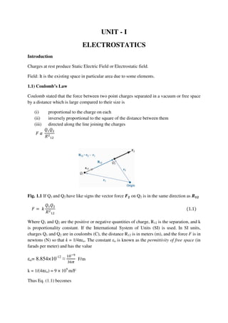
  • 1. UNIT - I ELECTROSTATICS Introduction Charges at rest produce Static Electric Field or Electrostatic field. Field: It is the existing space in particular area due to some elements. 1.1) Coulomb’s Law Coulomb stated that the force between two point charges separated in a vacuum or free space by a distance which is large compared to their size is (i) proportional to the charge on each (ii) inversely proportional to the square of the distance between them (iii) directed along the line joining the charges ‫ ߙ ܨ‬ ܳଵܳଶ ܴଶ ଵଶ Fig. 1.1 If Q1 and Q2 have like signs the vector force ࡲ૛ on Q2 is in the same direction as ࡾ૚૛ ‫ܨ‬ = ݇ ܳଵܳଶ ܴଶ ଵଶ (1.1) Where Q1 and Q2 are the positive or negative quantities of charge, R12 is the separation, and k is proportionality constant. If the International System of Units (SI) is used. In SI units, charges Q1 and Q2 are in coulombs (C), the distance R12 is in meters (m), and the force F is in newtons (N) so that k = 1/4πεo. The constant εo is known as the permittivity of free space (in farads per meter) and has the value εo= 8.854×10⁻¹² ≈ ଵ଴షవ ଷ଺గ F/m k = 1/(4πεo) = 9 × 10⁹ m/F Thus Eq. (1.1) becomes
  • 2. ‫ܨ‬ = 1 4ߨߝ௢ ܳଵܳଶ ܴଶ ଵଶ (1.2) If point charges Q1 and Q2 are located at points having position vectors ࢘૚ and ࢘૛, then the force F2 on Q1 due to Q2, shown in Figure 1.1, is given by ࡲ૛ = 1 4ߨߝ௢ ܳଵܳଶ ܴଶ ଵଶ ࢇࡾ૚૛ (1.3) Where ࢇࡾ૚૛ = ࡾ૚૛ |ࡾ૚૛| (1.4) ࡾ૚૛ = ࢘૛ − ࢘૚ ܴଵଶ = |ࡾ૚૛| By substituting eq. (1.4) into eq. (1.3), we may write eq. (1.3) as ࡲ૛ = 1 4ߨߝ௢ ܳଵܳଶ ܴଷ ଵଶ ࡾ૚૛ (1.5) It is worthwhile to note that The force ࡲ૚ on Q1 due to Q2 is given by ࡲ૚ = |ࡲ૛|ࢇࡾ૛૚ = |ࡲ૛|(−ࢇࡾ૚૛ ) = −ࡲ૛ ࡲ૚ = −ࡲ૛ (1.6) Problems 1. The charge Q2 = 10 µc is located at (3,1,0) and Q1 = 50 µc is located at (-1,1,-3). Find the force on Q1. Ans. R21 = (-1-3) i + (1-1) j + (-3-0) k = -4i-3k | R21| = ඥ(−4)ଶ + (−3)ଶ = 5 ࡲ૚ = 1 4ߨߝ௢ ܳଵܳଶ ܴଷ ଶଵ ࡾ૛૚ ࡲ૚ = 9 × 10ଽ 10 × 10ି଺ × 50 × 10ି଺ 5ଷ (−4i − 3k) ࡲ૚ = −૙. ૚૝૝ ࢏ − ૙. ૚૙ૡ ࢑ 2. A point charge Q1 = 300 µc located at (1,-1,-3) experiences a force F1= 8i-8j+4k due to a point charge Q2 at (3,-3,-2)m. Determine Q2. Ans. R21 = (1-3) i + (3-1) j + (2-3) k = -2 i +2 j - k
  • 3. | R21| = ඥ(−2)ଶ + (2)ଶ + (−1)ଶ = 3 ࡲ૚ = 1 4ߨߝ௢ ܳଵܳଶ ܴଷ ଶଵ ࡾ૛૚ (8i − 8j + 4k ) = 9 × 10ଽ ܳଶ × 300 × 10ି଺ 3ଷ (−2 i + 2 j − k) Q2 = -40 µc. 1.2) Force due to N no. of charges: If we have more than two point charges, we can use the principle of superposition to determine the force on a particular charge. The principle states that if there are N charges Q1, Q2, Q3..................... QN located, respectively, at points with position vectors ࢘૚, ࢘૛, ࢘૜ … … … … … ࢘ࡺ , the resultant force ࡲ on a charge Q located at point(p) ࢘ is the vector sum of the forces exerted on Q by each of the charges Q1, Q2, Q3..................... QN. Hence: ࡲ = ࡲ૚ + ࡲ૛ + ⋯ + ࡲࡺ ࡲ = 1 4ߨߝ௢ ܳܳଶ ܴଷ ଵ௣ ࡾ૚࢖ + 1 4ߨߝ௢ ܳܳଶ ܴଷ ଶ௣ ࡾ૛࢖ + ⋯ + 1 4ߨߝ௢ ܳܳଶ ܴଷ ே௣ ࡾࡺ࢖ (1.7) ࡲ = ܳ 4ߨߝ௢ ෍ ܳ௜ ܴଷ ௜௣ ࡾ࢏࢖ ே ௜ୀଵ (1.8) ࡲ = 9 × 10ଽ ܳ ෍ ܳ௜ ܴଷ ௜௣ ࡾ࢏࢖ ே ௜ୀଵ (1.9) Problems 1. Find the force on a 100 µc charge at (0,0,3)m. If four like charges of 20 µc are located on x and y axes at ±4m. Ans. R1p = (0-4) i + (0-0) j + (3-0) k = -4 i +3 k | R1p| = ඥ(−4)ଶ + (3)ଶ = 5 R2p = (0-0) i + (0-4) j + (3-0) k = -4 j +3 k | R2p| = ඥ(−4)ଶ + (3)ଶ = 5 R3p = (0+4) i + (0-0) j + (3-0) k = 4 i +3 k
  • 4. | R3p| = ඥ(4)ଶ + (3)ଶ = 5 R4p = (0-0) i + (0+4) j + (3-0) k = 4 i +3 k | R4p| = ඥ(4)ଶ + (3)ଶ = 5 ࡲ = 9 × 10ଽ ܳ ෍ ܳ௜ ܴଷ ௜௣ ࡾ࢏࢖ ே ௜ୀଵ ࡲ = 9 × 10ଽ 100 × 10ି଺ × 20 × 10ି଺ 5ଷ (−4 i + 3 k − 4 i + 3 k + 4 i + 3 k + 4 i + 3 k) ࡲ = ૚. ૠ૛ ࡷ ܰ 2. Two small diameter 10 gm dielectric balls can slide freely on a vertical plastic channel. Each ball carries a negative charge of 1 nc. Find the separation between the balls if the upper ball is restrained from moving. Ans. Gravitational force and coulomb force must be equal F2 = mg = 10 × 10-3 × 9.8 = 9.8× 10⁻² N. ‫ܨ‬ଵ = 1 4ߨߝ௢ ܳܳଶ ܴଶ ଵ௣ Therefore F1 = F2 9.8× 10-2 = ଽ×ଵ଴వ (ଵ× ଵ଴షల)మ ோమ R=0.302 m 1.3) Electric Field Intensity or Electric Field Strength (ࡱ): It is the force per unit charge when placed in electric field. Fig 1.2 The lines of force due to a pair of charges, one positive and the other negative
  • 5. Fig 1.3 The lines of force due to a pair of positive charges An electric field is said to exist if a test charge kept in the space surrounding another charge, then it will experience a force. Thus, ࡱ = lim ொ೟→଴ ࡲ࢚ ܳ௧ (1.10) or simply ࡱ = ࡲ࢚ ܳ௧ (1.11) The electric field intensity ࡱ is obviously in the direction of the force ࡲ and is measured in newton/coulomb or volts/meter. The electric field intensity at point ࢚࢘ due to a point charge located at ࢘૚ is readily obtained from eq. (1.3) as ࡲ࢚ = 1 4ߨߝ௢ ܳଵܳ௧ ܴଶ ଵ௧ ࢇࡾ૚࢚ ࡲ࢚ ܳ௧ = 1 4ߨߝ௢ ܳଵ ܴଶ ଵ௧ ࢇࡾ૚࢚ ࡱ = 1 4ߨߝ௢ ܳଵ ܴଶ ଵ௧ ࢇࡾ૚࢚ (1.12) 1.3.1) Electric field due to N no. of charges: If we have more than two point charges, we can use the principle of superposition to determine the force on a particular charge. The resultant force ࡲ on a charge Q located at point(p) ࢘ is the vector sum of the forces exerted on Q by each of the charges Q1, Q2, Q3..................... QN. Hence: ࡲ = ࡲ૚ + ࡲ૛ + ⋯ + ࡲࡺ From eq. (1.9)
  • 6. ࡲ = 9 × 10ଽ ܳ ෍ ܳ௜ ܴଷ ௜௣ ࡾ࢏࢖ ே ௜ୀଵ We know that ࡱ = ࡲ ܳ ࡱ = 9 × 10ଽ ෍ ܳ௜ ܴଷ ௜௣ ࡾ࢏࢖ ே ௜ୀଵ (1.13) 1.3.2) Electric Fields Due to Continuous Charge Distributions: So far we have only considered forces and electric fields due to point charges, which are essentially charges occupying very small physical space. It is also possible to have continuous charge distribution along a line, on a surface, or in a volume as illustrated in figure 1.2. Fig. 1.4 volume charge distribution and charge elements It is customary to denote the line charge density, surface charge density, and volume charge density by λ (in C/m), σ (in C/m2 ), and ρv (in C/m3 ), respectively. Line charge density: when the charge is distributed over linear element, then the line charge density is the charge per unit length. λ = lim ௗ௟→଴ ݀‫ݍ‬ ݈݀ where dq is the charge on a linear element dl. Surface charge density: when the charge is distributed over surface, then the surface charge density is the charge per unit area.
  • 7. σ = lim ௗ௦→଴ ݀‫ݍ‬ ݀‫ݏ‬ where dq is the charge on a surface element ds. Volume charge density: when the charge is confined within a volume, then the volume charge density is the charge per unit volume. ρ୴ = lim ௗ௩→଴ ݀‫ݍ‬ ݀‫ݒ‬ where dq is the charge contained in a volume element dv. 1.3.3) Electric field due to line charge: Consider a uniformly charged wire of length L m, the charge being assumed to be uniformly distributed at the rate of λ (linear charge density) c/m. Let P be any point at which electric field intensity has to be determined. Consider a small elemental length dx at a distance x meters from the left end of the wire, the corresponding charge element is λ dx. Divide the wire into a large number of such small elements, each element will render its contribution towards the production of field at P. Fig 1.5 Evaluation E due to line charge Let dE be field due to the charge element λ dx. It has a component dEx along x-axis and dEy along y-axis. dE = dEx ax + dEy ay
  • 8. we know that ݀‫ܧ‬ = λ dx 4ߨߝ௢‫ݎ‬ଶ (1.14) From figure 1.5 we can write, dEx = dE cosߠ (1.15) dEy = dE sinߠ (1.16) Therefore we can write, ݀‫ܧ‬௫ = λ cosθ dx 4ߨߝ௢‫ݎ‬ଶ (1.17) ݀‫ܧ‬௬ = λ sinθ dx 4ߨߝ௢‫ݎ‬ଶ (1.18) Substituting eqs. (1.17) and (1.18) in dE we get, ݀ࡱ = λ cosθ dx 4ߨߝ௢‫ݎ‬ଶ ࢇ࢞ + λ sinθ dx 4ߨߝ௢‫ݎ‬ଶ ࢇ࢟ (1.19) From figure 1.5 we write L1-x = h cotߠ (1.20) -dx = -h cosec2 ߠ dߠ (1.21) r = h cosecߠ (1.22) Substituting equations (1.20), (1.21) and (1.22) in 1.19, we get ݀ࡱ = λ cosθ dθ 4ߨߝ௢ℎ ࢇ࢞ + λ sinθ dθ 4ߨߝ௢ℎ ࢇ࢟ (1.23) The electric field intensity E due to whole length of the wire ࡱ = න ݀ࡱ ݀ߠ ࣂୀ࣊ିࢻ૛ ࣂୀࢻ૚ ࡱ = න ൤ λ cosθ dθ 4ߨߝ௢ℎ ࢇ࢞ + λ sinθ dθ 4ߨߝ௢ℎ ࢇ࢟ ൨ ݀ߠ ࣂୀ࣊ିࢻ૛ ࣂୀࢻ૚
  • 9. ࡱ = ߣ 4ߨߝ௢ℎ ൣ‫ࢇ ߠ݊݅ݏ‬࢞ − ܿ‫ࢇ ߠݏ݋‬࢟൧ ࢻ૚ ࣊ିࢻ૛ ࡱ = ߣ 4ߨߝ௢ℎ ൣ(‫ߙ݊݅ݏ‬ଶ − ‫ߙ݊݅ݏ‬ଵ)ࢇ࢞ + (ܿ‫ߙݏ݋‬ଶ + ܿ‫ߙݏ݋‬ଵ) ࢇ࢟൧ ܰ ‫ܥ‬ (1.24) Case (i) If P is the midpoint, α1= α2 = α ࡱ = ߣ 4ߨߝ௢ℎ ൣ(‫ߙ ݊݅ݏ‬ − ‫ࢇ)ߙ ݊݅ݏ‬࢞ + (ܿ‫ߙ ݏ݋‬ + ܿ‫ࢇ )ߙ ݏ݋‬࢟൧ ܰ ‫ܥ‬ ࡱ = ߣ 4ߨߝ௢ℎ ൣ2 ܿ‫ࢇ ߙ ݏ݋‬࢟൧ ܰ ‫ܥ‬ ࡱ = ߣ 2ߨߝ௢ℎ ܿ‫ࢇ ߙ ݏ݋‬࢟ ܰ ‫ܥ‬ (1.25) The direction of electric field intensity is normal to the line charge. The electric field is not normal to the line charge if the point is not at midpoint. Case (ii) As length tends to α1 = 0 and α2 = 0 from equation (1.24), we get ࡱ = ߣ 2ߨߝ௢ℎ ࢇ࢟ ܰ ‫ܥ‬ (1.26) 1.3.4) Electrical field due to charged ring: A circular ring of radius a carries a uniform charge λ C/m and is placed on the xy-plane with axis the same as the z-axis as shown in figure. Let dE be the electric field intensity due to a charge dQ. The ring is assumed to be formed by several point charges. When these vectors are resolved, radial components get cancelled and normal components get added. Therefore the direction of electric field intensity is normal to the plane of the ring. The sum of normal components can be written as ∞
  • 10. Fig. 1.6 charged ring ࡱ = න ݀‫ࢇ ߙݏ݋ܿ ܧ‬ࢠ ࡱ = න ݀ܳ 4ߨߝ௢ܴଶ ܿ‫ࢇ ߙ ݏ݋‬ࢠ ࡱ = න ߣ ݈݀ 4ߨߝ௢ܴଶ ℎ ܴ ࢇࢠ ࡱ = ߣ ℎ 4ߨߝ௢ܴଷ ࢇࢠ න ݈݀ ࡱ = ߣ ℎ 4ߨߝ௢ܴଷ × 2ߨܽ ࢇࢠ ࡱ = ߣ ℎ 4ߨߝ௢√ܽଶ + ℎଶ ଷ × 2ߨܽ ࢇࢠ ࡱ = ߣ ܽ ℎ 2ߝ௢(ܽଶ + ℎଶ)ଷ/ଶ ࢇࢠ N C (1.27)
  • 11. 1.3.5) Electrical field due to a charged disc: A disc of radius ‘a’ meters is uniformly charged with a charged density σ c/m2 . It is required to determine the electric field at ‘P’ which is at a distance h meters from the centre of the disc as shown in figure 1.7 Fig. 1.7 charged disc The disc is assumed to be formed by several rings of increasing radius. Consider a ring of radius x meters. Each ring is assumed to be formed by number of point charges. Let dE1 be the electric field intensity due to a charge dQ1 and dE2 is the electric field intensity due to a charge dQ2. Electric field due to one ring be obtained by adding normal components of dE1, dE2 ....... dEn. Therefore dE = (dE1 cosߠ + dE2 cosߠ + ....... + dEn cosߠ ) az dE = (dE1 + dE2 + ....... + dEn) cosߠ az dE = ( ௗொభ ସగఌ௥మ + ௗொమ ସగఌ௥మ + ....... + ௗொ೙ ସగఌ௥మ) cosߠ az dE = ௗொభାௗொమା⋯ାௗொ೙ ସగఌ௥మ cosߠ az dE = ௗொ ସగఌ௥మ cosߠ az The total charge of the ring is σ ds which is equal to dQ
  • 12. dE = σ ୢୱ ସగఌ௥మ cosߠ az (1.28) ds = π[(x + dx)2 – x2 ] ds = π[x2 + dx2 + 2xdx – x2 ] = 2π x dx (neglecting dx2 term) Substituting ds in eq. (1.28) , we get dE = σ ଶπ୶ୢ୶ ସగఌ௥మ cosߠ az dE = σ ୶ୢ୶ ଶఌ௥మ cosߠ az (1.29) From above figure we can write Tanߠ = x/h x = h tanߠ (1.30) dx = h sec2 ߠ dߠ (1.31) cosߠ = h/r r = h/ cosߠ = h secߠ (1.32) Substituting eqs. (1.30), (1.31) and (1.32) in (1.29) we get, dE = σ ( ୦ ୲ୟ୬θ)(୦ ୱୣୡమθ ୢθ) ଶఌ୦ ୱୣୡθమ cosߠ az dE = σ ଶఌ sinߠ dߠ az On integrating ࡱ = ߪ 2ߝ න ‫ߠ݊݅ݏ‬ ఈ ଴ ݀ߠ ࢇࢠ ࡱ = ߪ 2ߝ ሾ−ܿ‫ߠݏ݋‬ሿ଴ ఈ ࢇࢠ ࡱ = ߪ 2ߝ (1 − ܿ‫ࢇ)ߙݏ݋‬ࢠ (1.33) From figure 1.7 ܿ‫ߙݏ݋‬ = ℎ ඥ(ܽଶ + ℎଶ)
  • 13. ∴ ࡱ = ߪ 2ߝ ቆ1 − ℎ ඥ(ܽଶ + ℎଶ) ቇ ࢇࢠ ܰ ‫ܥ‬ (1.34) For infinite disc, radius ‘a’ tends to infinite and α = 90. ࡱ = ߪ 2ߝ (1 − ܿ‫ࢇ)09 ݏ݋‬ࢠ ࡱ = ߪ 2ߝ ࢇࢠ ܰ ‫ܥ‬ ‫ݎ݋‬ ܸ ݉ (1.35) From equation (1.35), it can be seen that electric field due to infinite disc is independent of distance. Electric field is uniform. Problems 1. Determine the magnitude of electric field at a point 3 cm away from the mid point of two charges of 10-8 c and -10-8 c kept 8 cm apart as shown in figure. Ans. Er = 2 |E| cos ߠ |E1|=|E2|=E ‫ܧ‬ = 1 4ߨߝ௢ ܳ ܴଶ ‫ܧ‬ = 1 4ߨ 8.854 × 10ିଵଶ 10ି଼ 0.05ଶ = 36 ‫ ݉/ܸ ܭ‬ Er = 2 36 × 103 cos 53.1 = 57.6 K V 2. A uniform charge distribution infinite in extent lies along z-axis with a charge density of 20 nc/m. Determine electric field intensity at (6,8,0). Ans. d = (6-0)i+(8-0)j+0 k = 6i + 8j d= ඥ(6ଶ + 8ଶ) = 10 ࡱ = ߣ 2ߨߝ௢݀ ࢇࢊ ܰ ‫ܥ‬ ࡱ = 20 × 10ିଽ 2ߨ 8.854 × 10ିଵଶ 10 6i + 8j 10 E = 21.57i + 28.76j N/C 3. A straight wire has an uniformly distributed charge of 0.3×10⁻⁴ c/m and of length 12 cm. Determine the electric field at a distance of 3 cm below the wire and displaced 3 cm to the right beyond one end as shown in figure. Ans. tan α1 = ஼௉ ஺஼ = ଴.଴ଷ ଴.ଵଶା଴.଴ଷ = ଴.଴ଷ ଴.ଵହ
  • 14. α1 = tan-1 (0.03/0.15)= 11.3o tan β = 0.03/0.03 = 1 β = 45o , α2 = 180-45= 135o ࡱ = ߣ 4ߨߝ௢ℎ ൣ(‫ߙ݊݅ݏ‬ଶ − ‫ߙ݊݅ݏ‬ଵ)ࢇ࢞ + (ܿ‫ߙݏ݋‬ଶ + ܿ‫ߙݏ݋‬ଵ) ࢇ࢟൧ ࡱ = 9 × 10ଽ × 0.3 × 10ିସ 0.03 ൣ(sin 135 − sin 11.3)ࢇ࢞ + (cos 135 + cos 11.3) ࢇ࢟൧ ࡱ = 4.59 × 10଺ ࢇ࢞ + 2.4 × 10଺ ࢇ࢟ ࡱ = ൫4.59 ࢇ࢞ + 2.4 ࢇ࢟൯ ‫ ݉/ݒܭ‬ 4. Find the force on a point charge 50 µc at (0,0,5) m due to a charge 0f 500π µc. It is uniformly distributed over a circular disc of radius 5 m. Ans. ߪ = ொ గ ௔మ ߪ = 500π 10ି଺ ߨ 5ଶ = 20 µ c/m ࡱ = ߪ 2ߝ (1 − ܿ‫ࢇ)ߙݏ݋‬ࢠ ࡱ = 20 × 10ି଺ 2 × 8.854 × 10ିଵଶ (1 − ܿ‫ࢇ )54 ݏ݋‬ࢠ ࡱ = 3.3 × 10ହ ࢇࢠ ܰ/‫ ܥ‬ F= E q F = 3.3 × 10ହ × 50 × 10ି଺ = 16.5 ܰ F = 16.5 az N 5. A charge of 40/3 nc is distributed around a ring of radius 2m, find the electric field at a point (0,0,5)m from the plane of the ring kept in Z=0 plane.
  • 15. Ans. Q = 40/3 n c ߣ = ܳ 2 ߨ ܽ = 40 3 × 10ିଽ 2 ߨ 2 = 1.06 × 10ିଽ ܿ ݉ ࡱ = ߣ ܽ ℎ 2ߝ௢‫ݎ‬ଷ ࢇࢠ N C ࡱ = 1.06 × 10ିଽ × 2 × 5 2 × 8.854 × 10ିଵଶ × √29 ଷ ࢇࢠ ࡱ = 3.83 ࢇࢠ ܸ 6. An infinite plane at y=3 m contains a uniform charge distribution of density 10-8 /6π C/m2 . Determine electric field at all points. Ans. (i) y>3 E = σ/2ϵ j = 10-8 /(2×6π×8.854×10-12 ) j = 29.959 j Magnitude of electric field at all points is same since the electric field due to an infinite plane (or) disc is uniform. For y<3 E = -29.959 j For y<3, electric field is directed along negative y-axis. Unit vector along negative y- direction is –j. 7. A straight line of charge of length 12 cm carries a uniformly distributed charge of 0.3×10⁻⁶ coulombs per cm length. Determine the magnitude and direction of the electric field intensity at a point (i) Located at a distance of a 3 cm above the wire displaced 3 cm to the right of and beyond one end. (ii) Located at the distance of 3 cm from one end, in alignment with, but beyond the wire. (iii) Located at a distance of 3 cm from one end, on the wire itself. ans. (i) tan α1 = ஼௉ ஺஼ = ଴.଴ଷ ଴.ଵଶା଴.଴ଷ = ଴.଴ଷ ଴.ଵହ α1 = tan-1 (0.03/0.15)= 11.3o tan β = 0.03/0.03 = 1 β = 45o , α2 = 180-45= 135o
  • 16. ࡱ = ߣ 4ߨߝ௢ℎ ൣ(‫ߙ݊݅ݏ‬ଶ − ‫ߙ݊݅ݏ‬ଵ)ࢇ࢞ + (ܿ‫ߙݏ݋‬ଶ + ܿ‫ߙݏ݋‬ଵ) ࢇ࢟൧ ࡱ = 9 × 10ଽ × 0.3 × 10ିସ 0.03 ൣ(sin 135 − sin 11.3)ࢇ࢞ + (cos 135 + cos 11.3) ࢇ࢟൧ ࡱ = 4.59 × 10଺ ࢇ࢞ + 2.4 × 10଺ ࢇ࢟ ࡱ = ൫4.59 ࢇ࢞ + 2.4 ࢇ࢟൯ ‫ ݉/ݒܭ‬ (ii) consider an element dx of charge λdx at a distance x from A. The field at P due to the positive charge element λdx is directed to the right. ࢊࡱ = ߣ݀‫ݔ‬ 4ߨߝ௢(‫ܮ‬ + ℎ − ‫)ݔ‬ଶ ࢇ࢞ ࡱ = ߣ 4ߨߝ௢ න ݀‫ݔ‬ (‫ܮ‬ + ℎ − ‫)ݔ‬ଶ ࡸ ଴ ࢇ࢞ ࡱ = ߣ 4ߨߝ௢ ൤ 1 ℎ − 1 ‫ܮ‬ + ℎ ൨ ࢇ࢞ ࡱ = 9 × 10ଽ × 0.3 × 10ିସ ൤ 1 0.03 − 1 0.15 ൨ ࢇ࢞ ࡱ = 7.2 × 10଺ ࢇ࢞ ࢜/࢓ (iii) Now L=AC= 6 cm = 0.06 cm h = 0.03 m ࡱ = ߣ 4ߨߝ௢ ൤ 1 ℎ − 1 ‫ܮ‬ + ℎ ൨ ࢇ࢞ ࡱ = 9 × 10ଽ × 0.3 × 10ିସ ൤ 1 0.03 − 1 0.09 ൨ ࢇ࢞
  • 17. E = 60 ax K v/cm 1.4) Work Done: If a point charge ‘Q’ is kept in an electric field it experience a force F in the direction of electric field. Fa is the applied force in a direction opposite to that of F. Let dw be the work done in moving this charge Q by a distance dl m. Total work done in moving the point charge from ‘a’ to ‘b’ can be obtained by integration. ܹ = න ݀‫ ݓ‬ ܹ = න ࡲࢇ ∙ ࢊ࢒ ܹ = − න ࡲ ∙ ࢊ࢒ ௕ ௔ (1.36) E = F/Q F = E Q ܹ = − න ࡱ ܳ ∙ ࢊ࢒ ௕ ௔ ܹ = −ܳ න ࡱ ∙ ࢊ࢒ ௕ ௔ (1.37) E = Ex ax + Ey ay + Ez az dl = dx ax + dyay + dz az E ∙ dl = EX dx + Ey dy + Ez dz ∴ ܹ = −ܳ න (E୶ dx + E୷ dy + E୸ dz) (௫మ,௬మ,௭మ) (௫భ,௬భ,௭భ) (1.38) Problems
  • 18. 1. Find the work involved in moving a charge of 1 c from (6,8,-10) to (3,4,-5) in the field E = -x i +y j –3 k. Ans. ܹ = −ܳ න (E୶ dx + E୷ dy + E୸ dz) (ଷ.ସ.ିହ) (଺,଼,ିଵ଴) ܹ = −1 ቈන −‫ݔ݀ ݔ‬ + ଷ ଺ න ‫ݕ݀ ݕ‬ ସ ଼ − න ‫ݖ݀ ݖ‬ ିହ ିଵ଴ ቉ ܹ = − ൥ቆ −‫ݔ‬ଶ 2 ቇ ଺ ଷ + ቆ ‫ݕ‬ଶ 2 ቇ ଼ ସ − (3‫)ݖ‬ିଵ଴ ିହ ൩ ܹ = − ൤ −9 2 + 36 2 + 16 2 − 64 2 − −15 + 30൨ W= 25.5 J 2. Find the work done in moving a point charge of -20 µc from the origin to (4,0,0) in the field E = (x/2 + 2y) i + 2x j Ans. ܹ = −ܳ න (E୶ dx + E୷ dy + E୸ dz) (௫మ,௬మ,௭మ) (௫భ,௬భ,௭భ) dl = d xi ܹ = −ܳ න (E୶ dx ) (ସ,଴,଴) (଴,଴,଴) ܹ = 20 × 10ି଺ න ((x/2 + 2y) dx ) (ସ,଴,଴) (଴,଴,଴) ܹ = 20 × 10ି଺ ቆ ‫ݔ‬ଶ 4 ቇ ଴ ସ W = 80×10-6 J 1.5) Absolute Potential: Absolute potential is defined as the work done in moving a unit positive charge from infinite to the point against the electric field.
  • 19. A point charge Q is kept at an origin as shown in figure. It is required to find the potential at ‘b’ which is at distance ‘r’ m from the reference. Consider a point R1 at a distance ‘x’ m. The small work done to move the charge from R1 to P1 is dw. The electrical field due to a point charge Q at a distance ‘x’ mis ࡱ = ܳ/(4ߨߝ‫ݔ‬ଶ ) Work done = E• dx Total work done can be obtained by integration Work done (W) = − Q ‫׬‬ ۳ ∙ d‫ܔ‬ ୠ ୟ V= − 1 ‫׬‬ ۳ ∙ d‫ܔ‬ ୠ ୟ V = − න ۳ ∙ d‫ܔ‬ ୠ ୟ E = Ex ax , dl = dx ax V = − න ܳ 4ߨߝ‫ݔ‬ଶ ݀‫ݔ‬ ୠ ୟ ܸ = ܳ 4ߨߝ‫ݎ‬ (1.39) 1.6) Potential Difference: Vab Potential difference Vab is defined as the work done in moving a unit positive charge from ‘b’ to ‘a’.
  • 20. Consider a point charge Q kept at the origin of a spherical co-ordinate system. The field is always in the direction of ar. No field in the direction of ߠ and ϕ. The points ‘a’ and ’b’ are at distance ra and rb respectively as shown in figure. Vୟୠ = − න ۳ ∙ d‫ܔ‬ ୟ ୠ E = Er ar , dl = dr ar Vୟୠ = − න E୰d୰ ୟ ୠ Vୟୠ = − න ܳ 4ߨߝ‫ݎ‬ଶ d୰ ୰౗ ୰ౘ Vୟୠ = ܳ 4ߨߝ ൤ 1 ‫ݎ‬௔ − 1 ‫ݎ‬௕ ൨ Vୟୠ = ܳ 4ߨߝ 1 ‫ݎ‬௔ − ܳ 4ߨߝ 1 ‫ݎ‬௕ Vୟୠ = Vୟ − ܸ௕ (1.40) 1.6.1) Potential difference due to line charge: The wire is uniformly charged with λ C/m. We have to find the potential difference Vab due to this line charge. Consider a point P at a distance P from the line charge.
  • 21. Fig. Line charge E = Eρ aρ dl = dρ aρ E•dl = Eρ aρ • dρ aρ = Eρ dρ Potential difference Vab is the work done in moving a unit +ve charge from ‘b’ to ‘a’. Vୟୠ = − න ۳ ∙ d‫ܔ‬ ୟ ୠ Vୟୠ = − න Eρ dρ ୟ ୠ Vୟୠ = − න ߣ 2ߨߝߩ dρ ρ౗ ρౘ Vୟୠ = ߣ 2ߨߝ ln ߩ௕ ߩ௔ (1.41) 1.6.2) Potential due to charged ring: A thin wire is bent in the form of a circular ring as shown in figure. It is uniformly charged with a charge density λ C/m. It is required to determine the potential at height ‘h’ m from the centre of the ring. The ring is assumed to be formed by several point charges. Fig. Charged ring Let dv be the potential due to the line charge element of length dl containing a charge dQ. ݀‫ݒ‬ = ݀ܳ 4ߨߝ‫ݎ‬ ݀‫ݒ‬ = ߣ݈݀ 4ߨߝ‫ݎ‬ ܸ = න ߣ݈݀ 4ߨߝ‫ݎ‬
  • 22. ܸ = ߣ 4ߨߝ‫ݎ‬ න ݈݀ ܸ = ߣ 4ߨߝ‫ݎ‬ 2ߨܽ ܸ = ߣܽ 2ߝ‫ݎ‬ ܸ = ߣܽ 2ߝ√ܽଶ + ܾଶ ‫)24.1( ݏݐ݈݋ݒ‬ 1.6.3) Potential due to a charged disc: let dv be the potential due to one ring. Each ring is assumed to be having several point charges dQ1, dQ2, ............ dQn. Potential due to the ring is the sum of potential. Fig. Charge disc ݀‫ݒ‬ = ݀ܳଵ 4ߨߝ‫ݎ‬ + ݀ܳଶ 4ߨߝ‫ݎ‬ + … … … … … . + ݀ܳ௡ 4ߨߝ‫ݎ‬ ݀‫ݒ‬ = ݀ܳଵ + ݀ܳଶ + … … . . + ݀ܳ௡ 4ߨߝ‫ݎ‬ ݀‫ݒ‬ = ݀ܳ 4ߨߝ‫ݎ‬ ݀‫ݒ‬ = ߪ ݀‫ݏ‬ 4ߨߝ‫ݎ‬ = ߪ 2ߨ‫ݔ݀ ݔ‬ 4ߨߝ‫ݎ‬ = ߪ ‫ݔ݀ ݔ‬ 2ߝ‫ݎ‬ Potential due to entire disc can be obtained by integration ܸ = න ݀‫ݒ‬ = න ߪ ‫ݔ݀ ݔ‬ 2ߝ‫ݎ‬ ௔ ଴ = ߪ 2ߝ න ‫ݔ‬ √‫ݔ‬ଶ + ℎଶ ௔ ଴ ݀‫ ݔ‬ Let ‫ݔ‬ଶ + ℎଶ = ‫ݐ‬ଶ 2x dx = 2t dt Therefore we have
  • 23. ܸ = ߪ 2ߝ න ‫ݐ݀ ݐ‬ ‫ݐ‬ √௔మା௛మ ௛ ܸ = ߪ 2ߝ න ݀‫ݐ‬ √௔మା௛మ ௛ ܸ = ߪ 2ߝ ቀඥܽଶ + ℎଶ − ℎቁ ‫)34.1( ݏݐ݈݋ݒ‬ At the centre of the disc , h=0; ܸ = ߪܽ 2ߝ ‫)44.1( ݏݐ݈݋ݒ‬ Problems 1. Find the work done in moving a poimt charge Q= 5 µ c from origin to (2m, π/4 , π/2), spherical co-ordinates in the field E = 5 e-r/4 ar + (10/(r sin θ)) aϕ v/m. Ans. dl = dr ar + rdθ aθ + r sinθ dϕ aϕ E• dl = 5 e-r/4 dr + 10 dϕ W = − Q න ۳ ∙ d‫ܔ‬ ୠ ୟ W = − 5 × 10ି଺ ቈන 5 eି୰/ସ dr ଶ ଴ න 10 dϕ π/ଶ ଴ ቉ W= -117.9 µ J. 2. 5 equal, point charges of 20 nc are located at x=2,3,4,5 and 6 cm. Determine the potential at the origin. Ans. By superposition principal V= V1 + V2 + V3 + V4 + V5 ܸ = ܳ 4ߨߝ‫ݎ‬ଵ + ܳ 4ߨߝ‫ݎ‬ଶ + ܳ 4ߨߝ‫ݎ‬ଷ + ܳ 4ߨߝ‫ݎ‬ସ + ܳ 4ߨߝ‫ݎ‬ହ
  • 24. ܸ = 20 × 10ି଻ 4ߨߝ௢ ൬ 1 2 + 1 3 + 1 4 + 1 5 + 1 6 ൰ = 261 ‫ ݏݐ݈݋ݒ‬ 3. A line charge of 0.5 nc/m lies along z-axis. Find Vab if a is (2,0,0) , and b is (4,0,0). Ans. Vୟୠ = ߣ 2ߨߝ ln ߩ௕ ߩ௔ Vୟୠ = 0.5 × 10ିଽ 2ߨ × 8.854 × 10ିଵଶ ln 4 2 Vab = 6.24 V. 4. A point charge of 0.4 nc is located at (2,3,3) in Cartesian coordinates. Find Vab if a is (2,2,3) and b is (-2,3,3). Ans. Vୟୠ = Vୟ − ܸ௕ Vୟୠ = ܳ 4ߨߝ 1 ‫ݎ‬௔ − ܳ 4ߨߝ 1 ‫ݎ‬௕ ra = (2-2) i + (2-3) j + (3-3) k = -j ra = 1 rb = (-2-2) i + (3-3) j + (3-3) k = -4 i rb = 4 Vୟୠ = 0.4 × 10ିଽ 4ߨ × 8.854 × 10ିଵଶ ൤ 1 1 − 1 4 ൨ = 2.7 ‫ ݒ‬ 5. A total charge of 40/3 nc is distributed around a ring of radius 2m. Find the potential at a point on the z-axis 5m from the plane of the ring kept at z=0. What would be the potential if the entire charge is concentrated at the centre. ans. ܸ = ߣܽ 2ߝ√ܽଶ + ܾଶ ‫ ݏݐ݈݋ݒ‬ ߣ = ܳ ݈ = 40 3 × 10ିଽ 2ߨ 2 = 1.06 × 10ିଽ ‫ܥ‬ ݉
  • 25. ܸ = 1.06 × 10ିଽ × 2 2 × 8.854 × 10ିଵଶ × √2ଶ + 5ଶ = 22.2 ‫ ݒ‬ 6. Determine the potential at (0,0,5)m due to a total charge of 10-8 c distributed uniformly along a disc of radius 5m lying in the Z=0 plane and centered at the orign. Ans. ܸ = ߪ 2ߝ ቀඥܽଶ + ℎଶ − ℎቁ ‫ ݏݐ݈݋ݒ‬ ߪ = ܳ ܽ‫ܽ݁ݎ‬ = 10ି଼ ߨ × 5ଶ ܸ = 10ି଼ ߨ × 5ଶ 2ߝ ቀඥ5ଶ + 5ଶ − 5ቁ V= 14.89 v 1.7) Relation between V and E: Consider a point charge Q at the origin as shown in figure. Electric field due to this charge at the point ‘P’ is ࡱ = ܳ 4ߨߝ‫ݎ‬ଶ ࢇ࢘ Consider સ ൬ 1 ‫ݎ‬ ൰ = ൬ ߲ ߲‫ݎ‬ ࢇ࢘ + … … … ൰ ൬ 1 ‫ݎ‬ ൰ સ ൬ 1 ‫ݎ‬ ൰ = − ൬ 1 ‫ݎ‬ଶ ൰ ࢇ࢘ Using above expression in E , we get ࡱ = ܳ 4ߨߝ − સ ൬ 1 ‫ݎ‬ ൰ ࡱ = −સ ܳ 4ߨߝ ൬ 1 ‫ݎ‬ ൰ Therefore, ࡱ = −સ ܸ
  • 26. Problem 1. Given V= (x-2)2 × (y+2)2 ×(z-1)3 . Find electric field at the origin. Ans. V= (x-2)2 × (y+2)2 ×(z-1)3 ࡱ = −સ ܸ ࡱ = − ൬ ∂v ∂x i + ∂v ∂y j + ∂v ∂z k൰ ࡱ = −2(x − 2)× (y+2)2 ×(z-1)3 i-(x-2)2 × 2(y+2) ×(z-1)3 j - (x-2)2 × (y+2)2 ×3(z-1)2 k Electric field at the origin ࡱ = −2(0 − 2) (0+2)2 ×(0-1)3 i -(0-2)2 × 2(0+2) ×(0-1)3 j - (0-2)2 × (0+2)2 ×3(0-1)2 k E = -(16i+16j+48k) v/m. 1.8) Poisson’s and Laplace’s Equations: From the Gauss law we know that ‫׬‬ ‫.ܦ‬ ݀‫ݏ‬ = Q (1) A body containing a charge density ρ uniformly distributed over the body. Then charge of that body is given by Q = ‫׬‬ ૉ ݀‫ݒ‬ (2) ‫׬‬ ‫.ܦ‬ ݀‫ݏ‬ = ‫׬‬ ૉ ݀‫ݒ‬ (3) This is integral form of Gauss law. As per the divergence theorem ‫׬‬ ‫.ܦ‬ ݀‫ ݏ‬ = ‫׬‬ સ. ۲ ݀‫ݒ‬ (4) સ. ۲ = ૉ (5) This is known as point form or vector form or polar form. This is also known as Maxwell’s first equation. D = ƐE (6) સ. ƐE = ρ સ. E = ࣋/Ɛ (7) We know that E is negative potential medium
  • 27. E = -સ‫܄‬ (8) From equations 7 and 8 સ. (– સ‫)܄‬ = ࣋/Ɛ સ2 V = - ࣋/Ɛ (9) Which is known as Poisson’s equation in static electric field. Consider a charge free region (insulator) the value of ρ = 0, since there is no free charges in dielectrics or insulators. સ2 V = 0 This is known as Laplace’s equation.