
The 2022 Mw 6.1 Pasaman Barat, Indonesia Earthquake, Confirmed the Existence of the Talamau Segment Fault Based on Teleseismic and Satellite Gravity Data
 ,
,  ,
,
Abstract
:1. Introduction
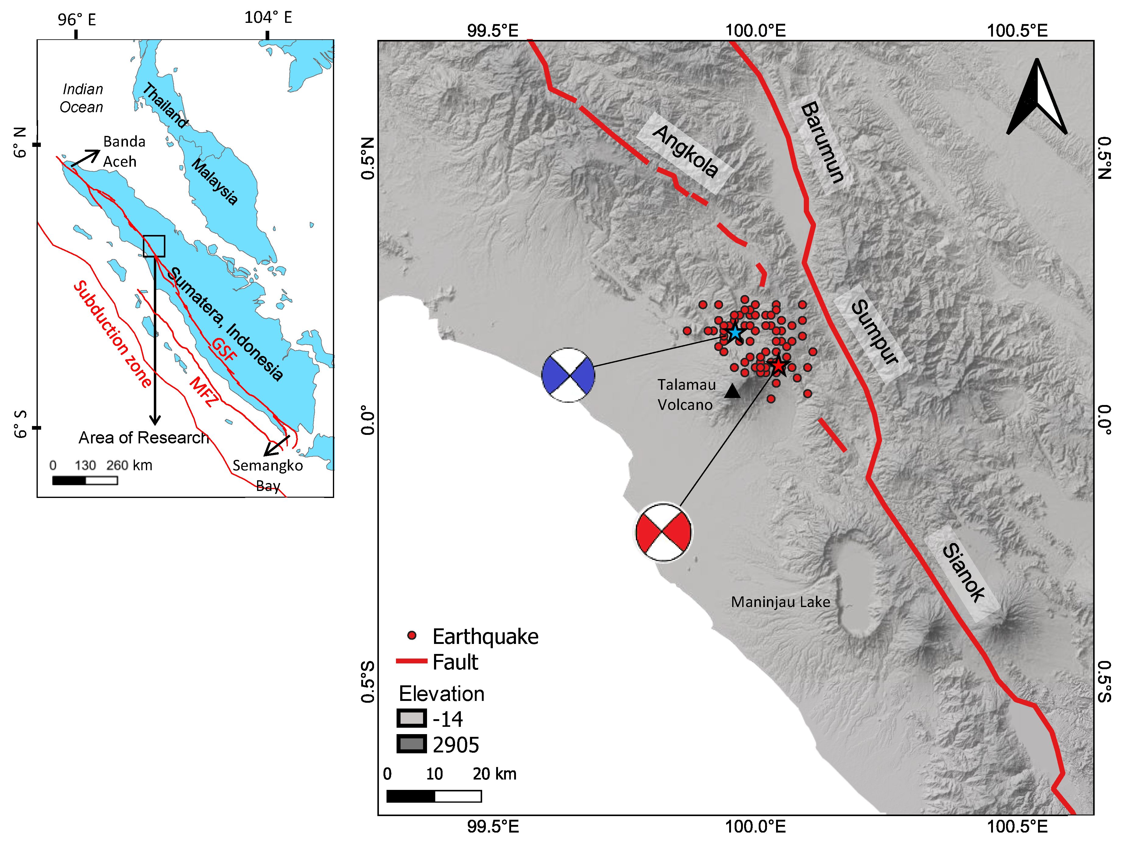
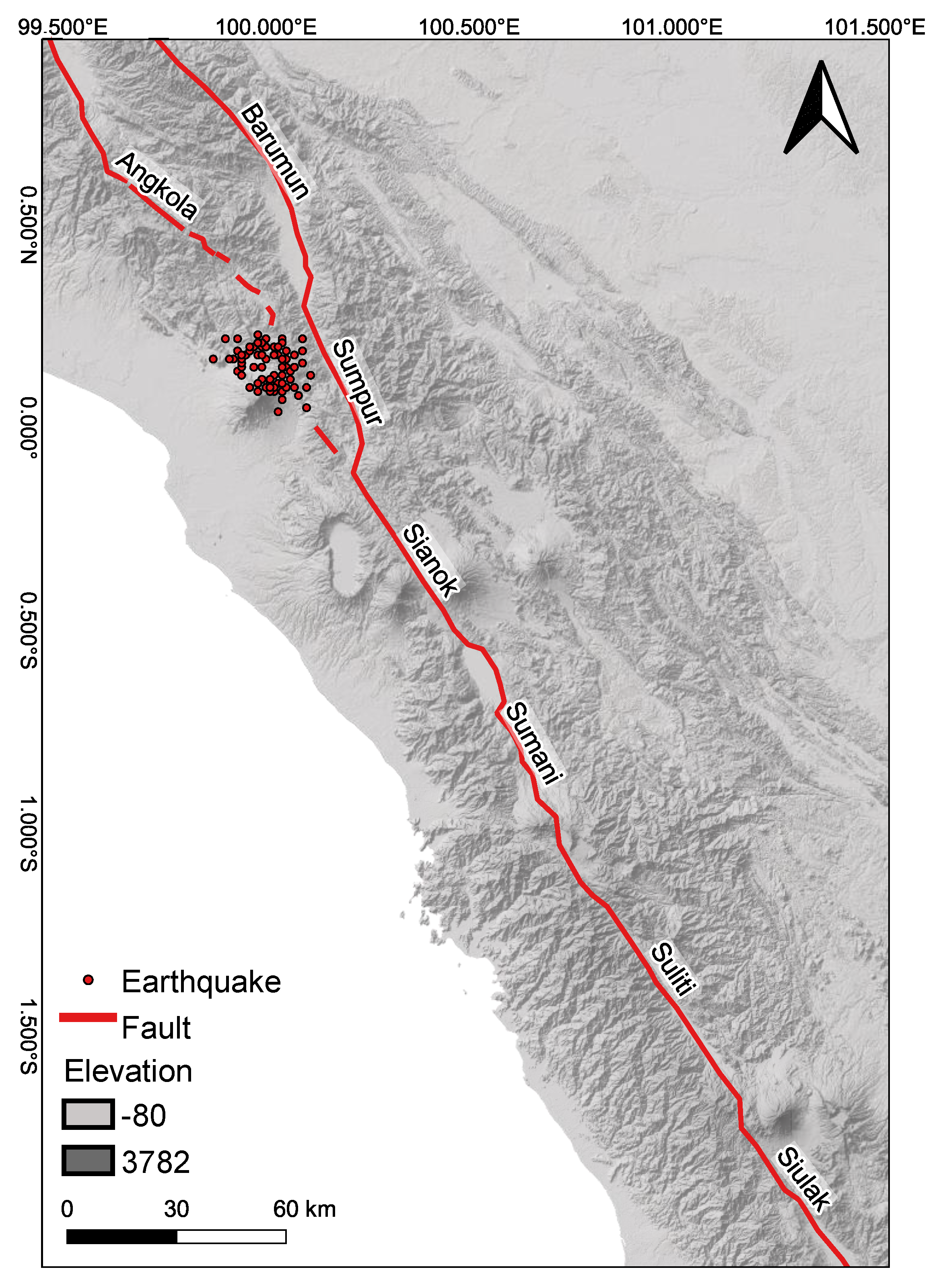
2. Study Area
2.1. Focus of Study Area
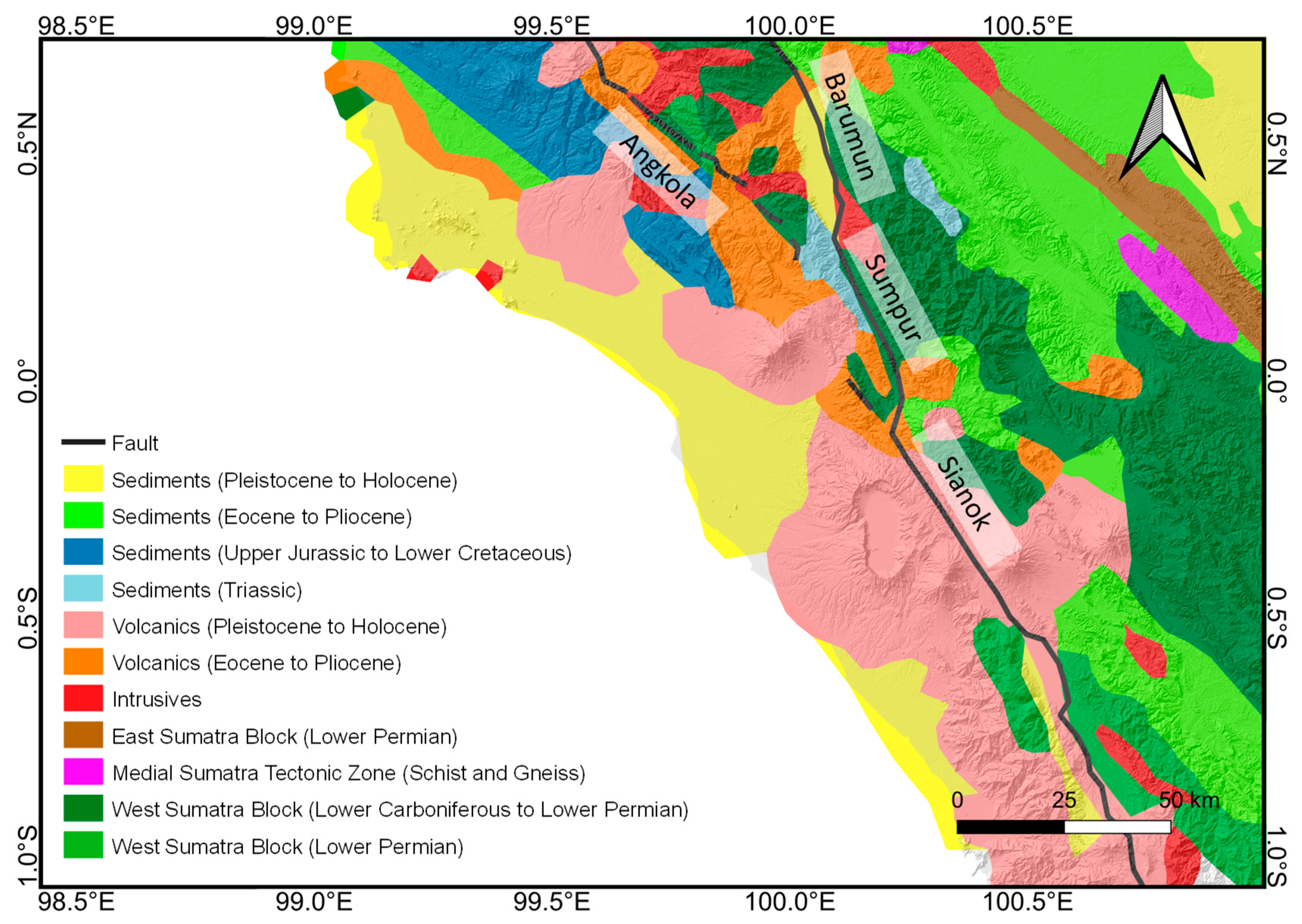
2.2. Geological Setting
3. Materials and Methods
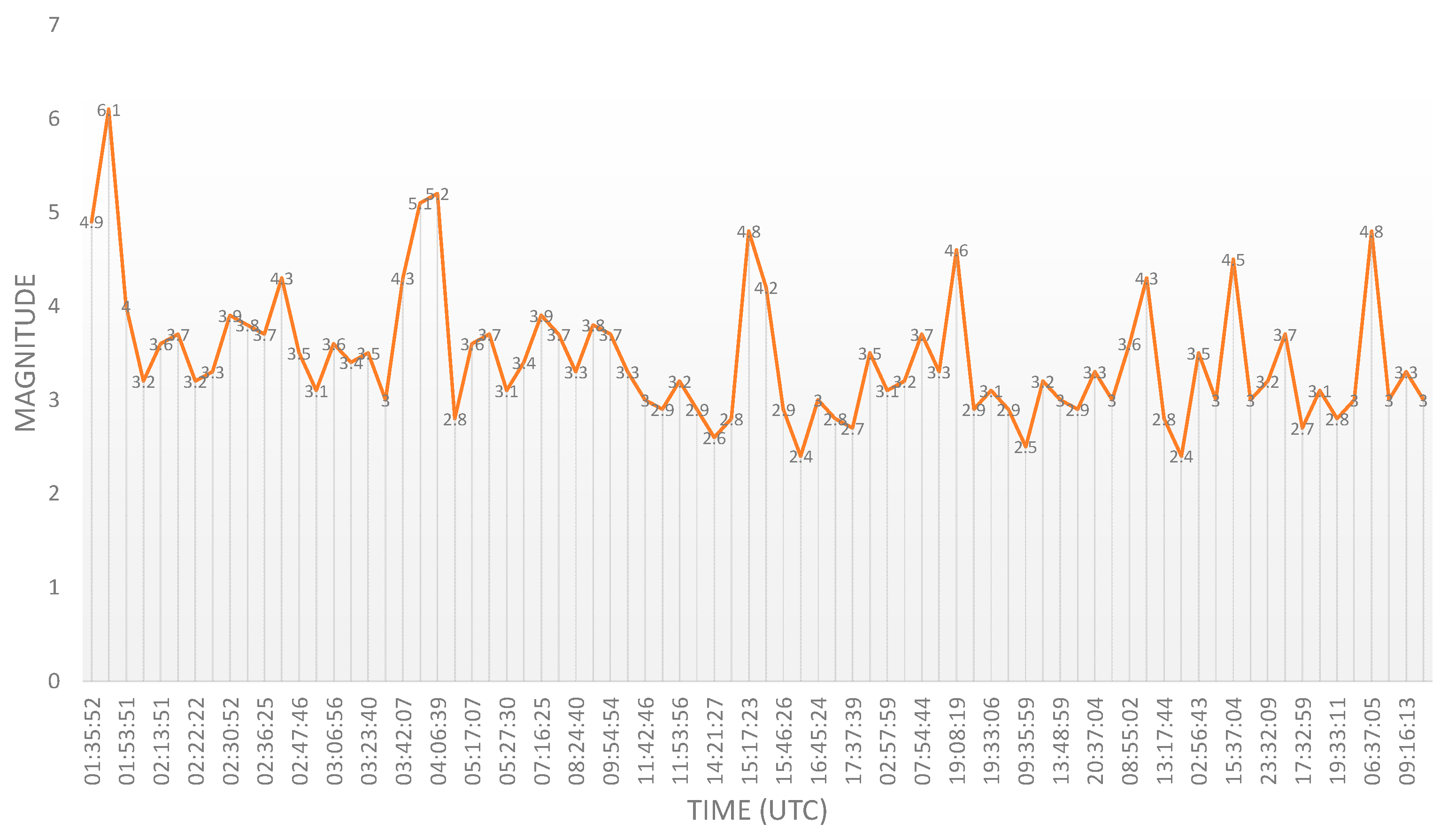
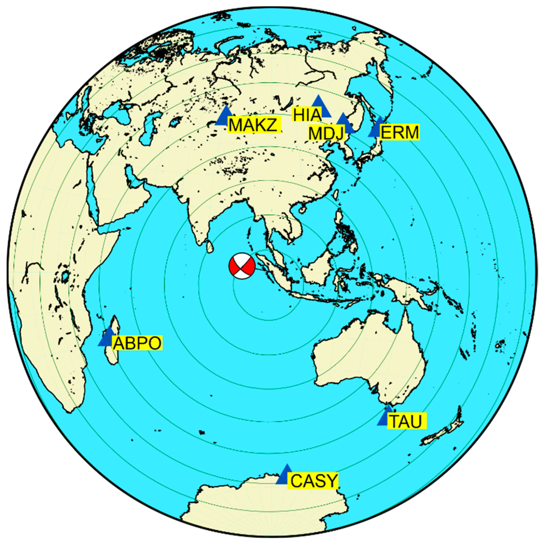
3.1. Teleseismic Data
3.2. Satellite Gravity Data
4. Results
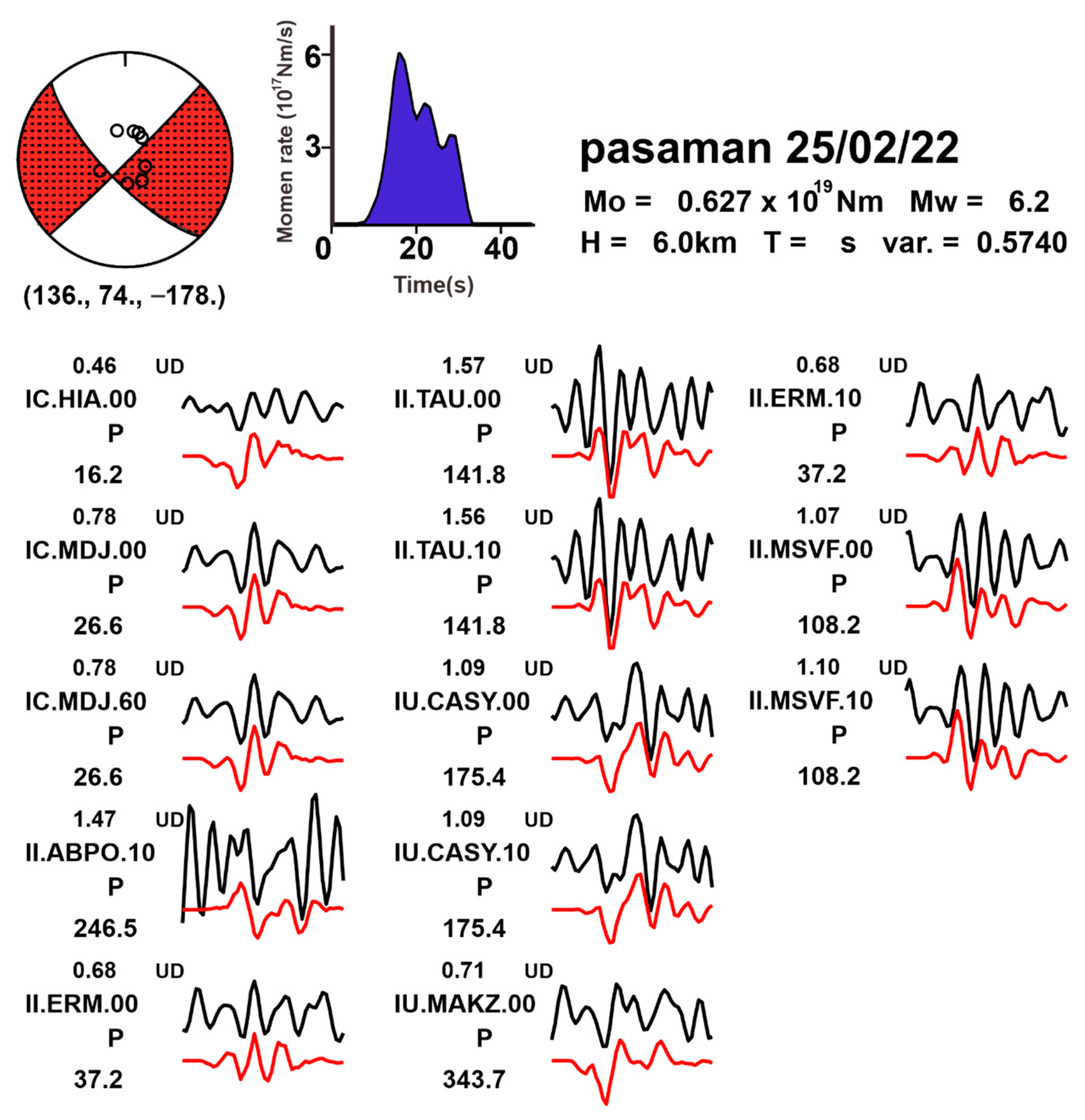
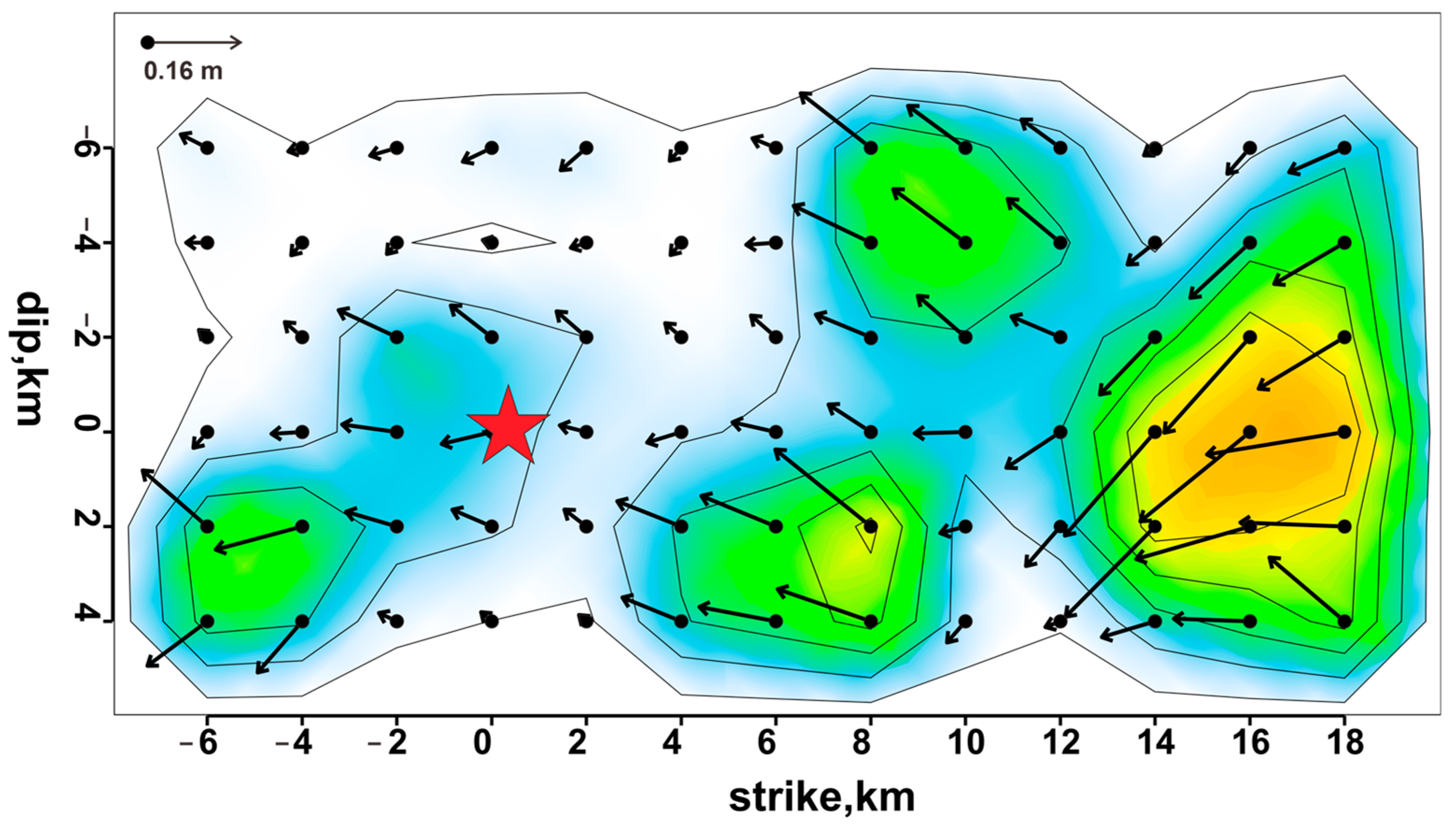
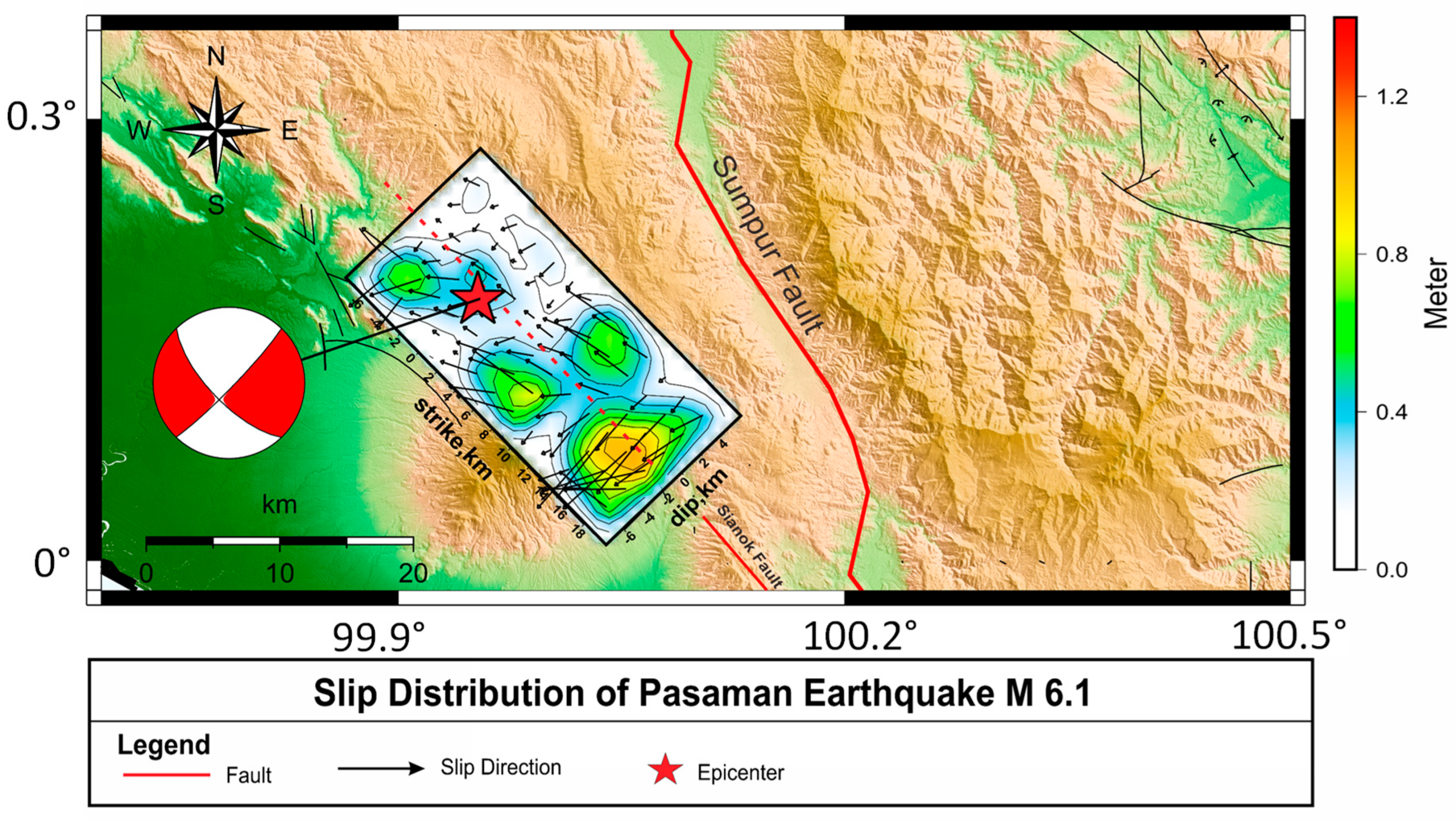
4.1. Coseismic Source Model Based on Teleseismic Data
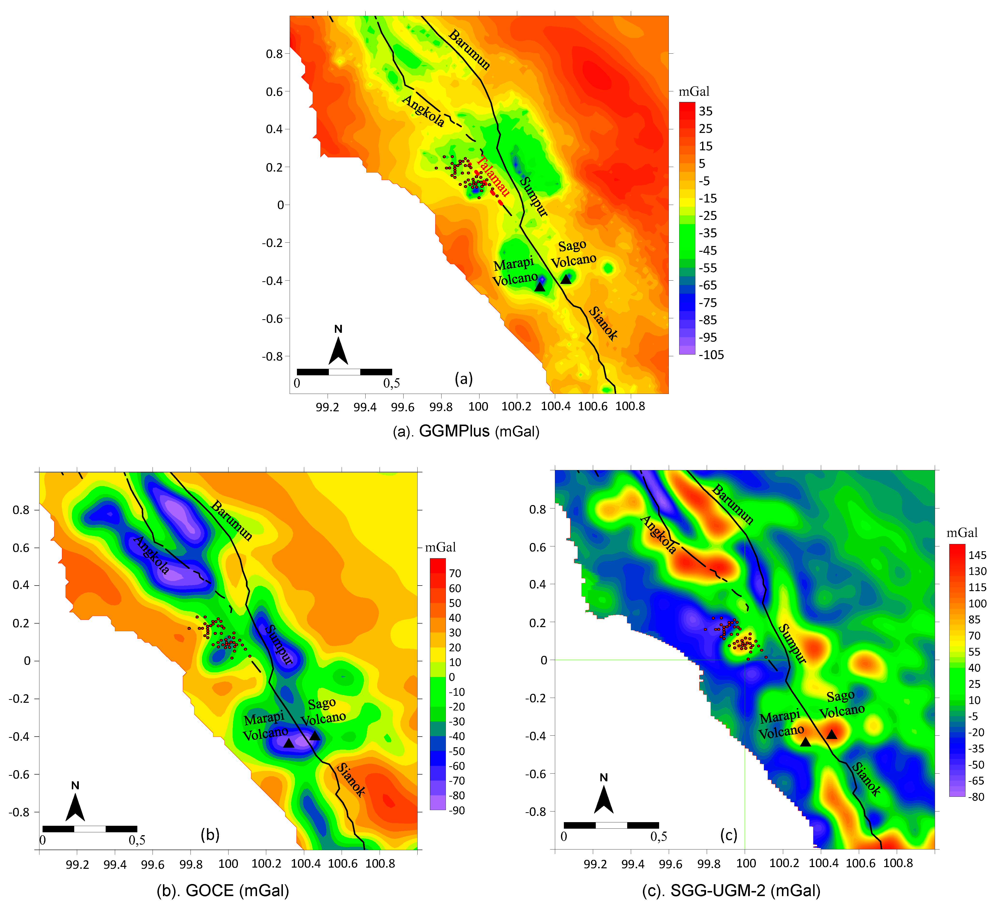
4.2. Fault Detection from Satellite Gravity Data
4.2.1. Simple Bouguer Anomaly (SBA)
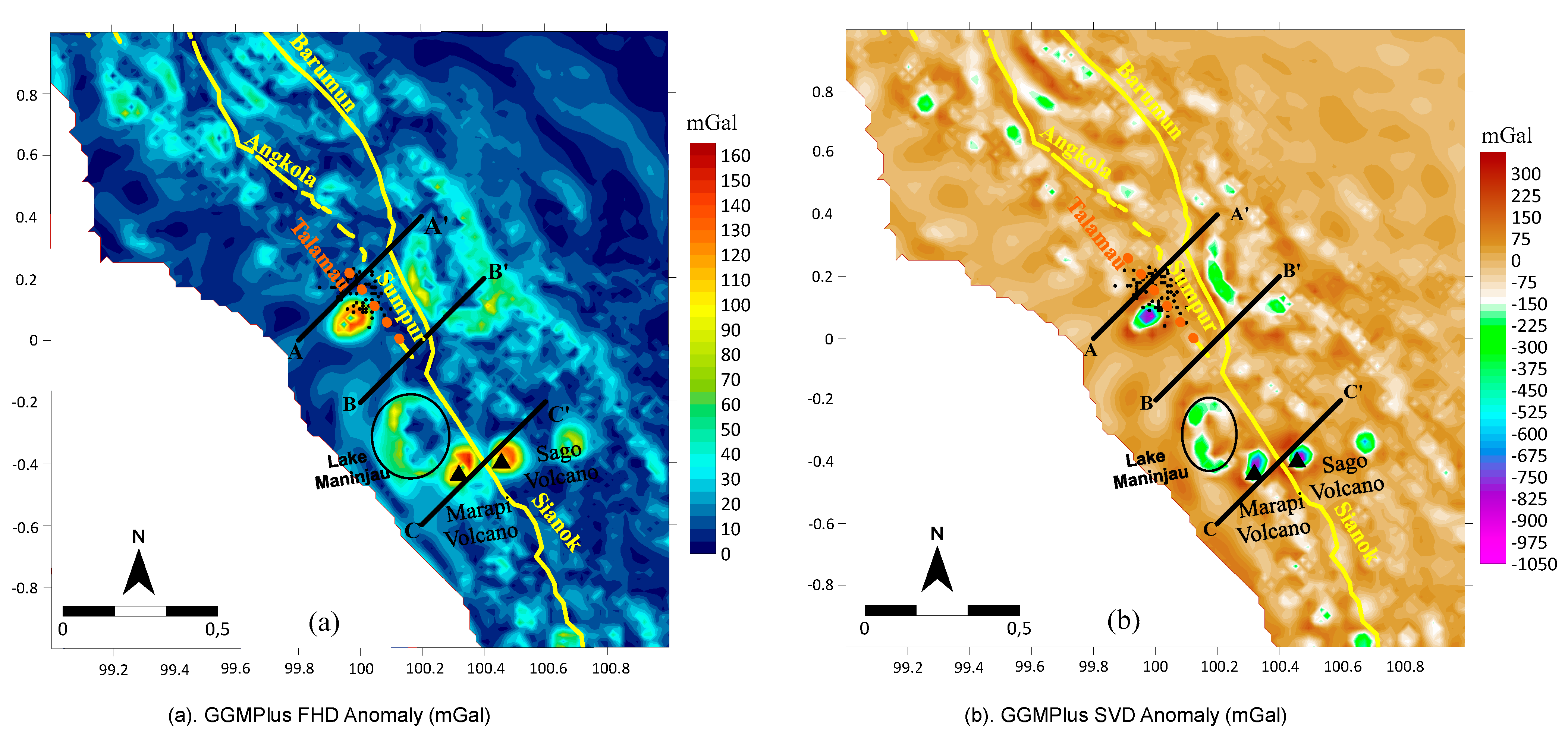
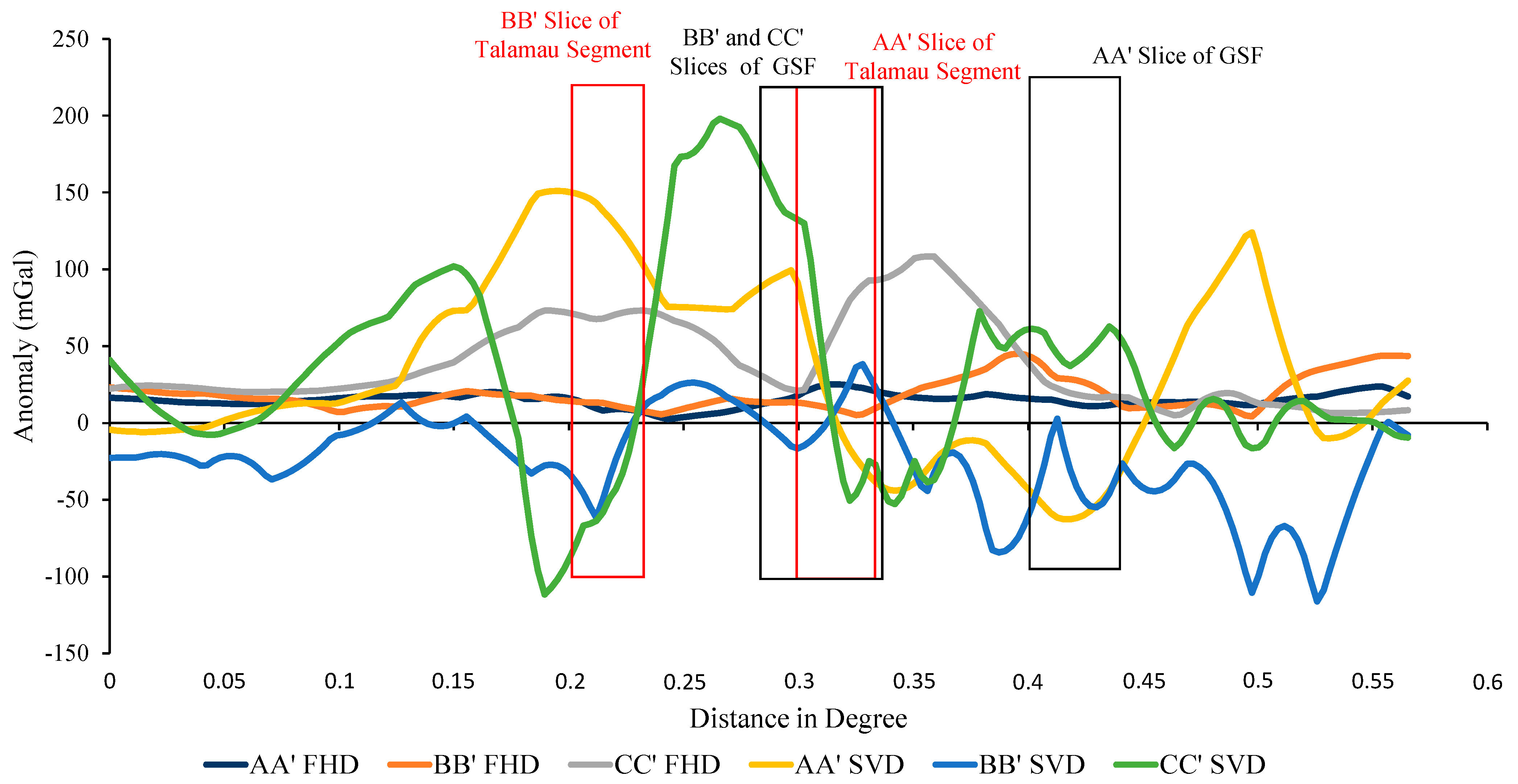
4.2.2. Data Transformation
5. Discussion
6. Conclusions
Author Contributions
Funding
Institutional Review Board Statement
Informed Consent Statement
Data Availability Statement
Acknowledgments
Conflicts of Interest
References
- Bellier, O.; Sébrier, M.; Pramumijoyo, S.; Beaudouin, T.; Harjono, H.; Bahar, I.; Forni, O. Paleoseismicity and Seismic Hazard Along the Great Sumatran Fault (Indonesia). J. Geod. 1997, 24, 169–183. [Google Scholar] [CrossRef]
- Noda, A. Strike-Slip Basin–Its Configuration and Sedimentary Facies. In Mechanism of Sedimentary Basin Formation-Multidisciplinary Approach on Active Plate Margins; IntechOpen: London, UK, 2013. [Google Scholar] [CrossRef] [Green Version]
- Natawidjaja, D.H.; Bradley, K.; Daryono, M.R.; Aribowo, S.; Herrin, J. Late Quaternary Eruption of the Ranau Caldera and New Geological Slip Rates of the Sumatran Fault Zone in Southern Sumatra, Indonesia. Geosci. Lett. 2017, 4, 21. [Google Scholar] [CrossRef] [Green Version]
- Acocella, V.; Bellier, O.; Sandri, L.; Sébrier, M.; Pramumijoyo, S. Weak Tectono-Magmatic Relationships Along an Obliquely Convergent Plate Boundary: Sumatra, Indonesia. Front. Earth Sci. 2018, 6, 3. [Google Scholar] [CrossRef] [Green Version]
- Muraoka, H.; Takahashi, M.; Sundhoro, H.; Dwipa, S.; Soeda, Y.; Momita, M.; Shimada, K. Geothermal Systems Constrained by the Sumatran Fault and Its Pull-Apart Basins in Sumatra, Western Indonesia. In Proceedings of the World Geothermal Congress 2010, Bali, Indonesia, 25–30 April 2010. [Google Scholar]
- Aydin, A.; Nur, A. Evolution of Pull-Apart Basins and Their Scale Independence. Tectonics 1982, 1, 91–105. [Google Scholar] [CrossRef]
- Natawidaja, D.H.; Triyoso, W. The Sumatran Fault Zone–From Source to Hazard. J. Earthq. Tsunami 2007, 1, 21–47. [Google Scholar] [CrossRef]
- Sieh, K.; Natawidjaja, D. Neotectonics of the Sumatran Fault, Indonesia. J. Geophys. Res. 2000, 105, 28295–28326. [Google Scholar] [CrossRef] [Green Version]
- Rock, N.M.S.; Aldiss, D.T.; Aspden, J.A.; Clarke, M.C.G.; Djunuddin, A.; Kartawa, W.; Miswar, T.S.J.; Whandoyo, R. Geologic Map of the Lubuksikaping Quadrangle, Sumatra; Geological Research and Development Centre: Bandung, Indonesia, 1983. [Google Scholar]
- Allen, R.M.; Ziv, A. Application of Real-Time GPS to Earthquake Early Warning. Geophys. Res. Lett. 2011, 38, L16310. [Google Scholar] [CrossRef]
- Hreinsdóttir, S.; Freymueller, J.T.; Bürgmann, R.; Mitchell, J. Coseismic Deformation of the 2002 Denali Fault Earthquake: Insights from GPS Measurements. J. Geophys. Res. 2006, 111, B03308. [Google Scholar] [CrossRef]
- Yamanaka, Y.; Kikuchi, M. Asperity Map Along the Subduction Zone in Northeastern Japan Inferred from Regional Seismic Data. J. Geophys. Res. 2004, 109, B07307. [Google Scholar] [CrossRef]
- Murotani, S.; Satake, K.; Fujii, Y. Scaling Relations of Seismic Moment, Rupture Area, Average Slip, and Asperity Size for M~9 Subduction-Zone Earthquakes. Geophys. Res. Lett. 2013, 40, 5070–5074. [Google Scholar] [CrossRef]
- Lo, W.; Purnomo, S.N.; Dewanto, B.G.; Sarah, D.; Sumiyanto. Integration of Numerical Models and InSAR Techniques to Assess Land Subsidence Due to Excessive Groundwater Abstraction in the Coastal and Lowland Regions of Semarang City. Water 2022, 14, 201. [Google Scholar] [CrossRef]
- Dewanto, B.G.; Haryanto, Y.; Purnomo, S.N. Land Subsidence Potential Detection in Yogyakarta International Airport Using Sentinel-1 Insar Data. Civ. Eng. Dimens. 2021, 23, 91–99. [Google Scholar] [CrossRef]
- Kikuchi, M.; Nakamura, M.; Yoshikawa, K. Source Rupture Processes of the 1944 Tonankai Earthquake and the 1945 Mikawa Earthquake Derived from Low-Gain Seismograms. Earth Planet Sp. 2003, 55, 159–172. [Google Scholar] [CrossRef] [Green Version]
- Sandwell, D.T.; Smith, W.H.F. Marine Gravity Anomaly from Geosat and ERS 1 Satellite Altimetry. J. Geophys. Res. 1997, 102, 10039–10054. [Google Scholar] [CrossRef] [Green Version]
- Kern, M.; Schwarz, K.P.; Sneeuw, N. A Study on the Combination of Satellite, Airborne, and Terrestrial Gravity Data. J. Geod. 2003, 77, 217–225. [Google Scholar] [CrossRef]
- Zhang, Y.-Z.; Xu, H.-J.; Wang, W.-D.; Duan, H.-R.; Zhang, B.-P. Gravity Anomaly from Satellite Gravity Gradiometry Data by GOCE in Japan Ms 9.0 Strong Earthquake Region. Procedia Environ. Sci. 2011, 10, 529–534. [Google Scholar] [CrossRef] [Green Version]
- Hirt, C.; Claessens, S.; Fecher, T.; Kuhn, M.; Pail, R.; Rexer, M. New Ultrahigh-Resolution Picture of Earth’s Gravity Field. Geophys. Res. Lett. 2013, 40, 4279–4283. [Google Scholar] [CrossRef] [Green Version]
- Hirt, C. Prediction of Vertical Deflections from High-Degree Spherical Harmonic Synthesis and Residual Terrain Model Data. J. Geod. 2010, 84, 179–190. [Google Scholar] [CrossRef] [Green Version]
- Hirt, C.; Kuhn, M.; Claessens, S.; Pail, R.; Seitz, K.; Gruber, T. Study of the Earth’s Short-Scale Gravity Field Using the ERTM2160 Gravity Model. Geosci. Comput. 2014, 73, 71–80. [Google Scholar] [CrossRef]
- Wada, S.; Sawada, A.; Hiramatsu, Y.; Matsumoto, N.; Okada, S.; Tanaka, T.; Honda, R. Continuity of Subsurface Fault Structure Revealed by Gravity Anomaly: The Eastern Boundary Fault Zone of the Niigata Plain, Central Japan. Earth Planets Sp. 2017, 69, 15. [Google Scholar] [CrossRef] [Green Version]
- Riedel, S.; Jokat, W.; Steinhage, D. Mapping Tectonic Provinces with Airborne Gravity and Radar Data in Dronning Maud Land, East Antarctica. Geophys. J. Int. 2012, 189, 414–427. [Google Scholar] [CrossRef] [Green Version]
- Hiramatsu, Y.; Sawada, A.; Kobayashi, W.; Ishida, S.; Hamada, M. Gravity Gradient Tensor Analysis to an Active Fault: A Case Study at the Togi-Gawa Nangan Fault, Noto Peninsula, Central Japan. Earth Planets Sp. 2019, 71, 107. [Google Scholar] [CrossRef]
- Yanis, M.; Abdullah, F.; Zaini, N.; Ismail, N. The Northernmost Part of the Great Sumatran Fault Map and Images Derived from Gravity Anomaly. Acta Geophys. 2021, 69, 795–807. [Google Scholar] [CrossRef]
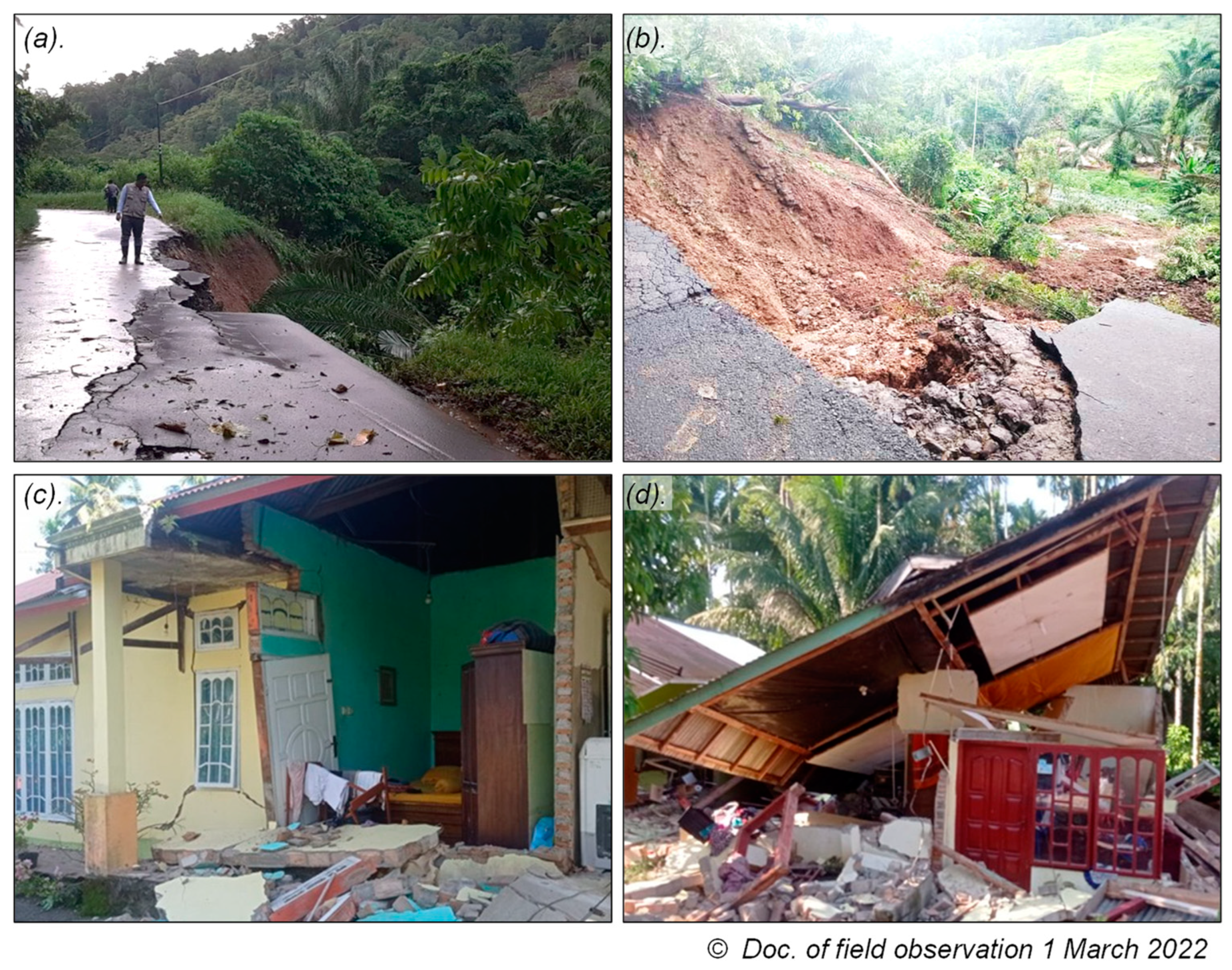
- Julius, A.M.; Pribadi, S.; Saputra, A.A.; Prayitno, B.S.; Ahadi, S.; Hermanto, D.; Arifin, H.; Satria, L.A.; Zevanya, C.S.S. An On-Site Post-Event Survey of the 2022 Mw 6.1 Western Pasaman Sumatera Destructive Earthquake. NTU J. Renew. Energy 2022, 2, 39–49. [Google Scholar]
- Kardo, R.; Mulyani, R.R.; Yulastri, W. Play Therapy as a Trauma Healing Effort in Children Victims of the Earthquake in Nagari Pasaman. J. Community Public Serv. 2022, 1, 90–94. [Google Scholar]
- Irkani, P.; Antomi, Y.; Yulfa, A.; Purwaningsih, E.; Triyatno. Visualisasi Potensi Daerah Kabupaten Pasaman Barat dalam Format Multimedia. 2010. Available online: repository.unp.ac.id/5919/1/PAUS%20ISKARNI_546_10.pdf (accessed on 5 April 2022).
- Iskarni, P.; Antomi, Y.; Yulfa, A.; Purwaningsih, E.; Triyatno. Visualization of the Potential of West Pasaman Regency in Multi Media Format; Regional Development Planning Agency, West Pasaman Regency Government in Collaboration with the Padang State University Spatial Data Infrastructure Development Center: Padang, Indonesia, 2010. [Google Scholar]
- Hall, R. Late Jurassic–Cenozoic Reconstructions of The Indonesian Region and The Indian Ocean. Tectonophysics 2012, 570–571, 1–41. [Google Scholar] [CrossRef] [Green Version]
- Barber, A.J.; Crow, M.J. Structure of Sumatra and its Implications for the Tectonic Assembly of Southeast Asia and the Destruction of Paleotethys. Island Arc. 2009, 18, 3–20. [Google Scholar] [CrossRef]
- Ghosal, D.; Singh, S.C.; Chauhan, A.P.S.; Hananto, N.D. New Insights on the Offshore Extension of the Great Sumatran Fault, NW Sumatra, from Marine Geophysical Studies. Geochem. Geophys. Geosyst. 2012, 13, Q0AF06. [Google Scholar] [CrossRef]
- De Maisonneuve, C.B.; Bergal-Kuvikas, O. Timing, Magnitude and Geochemistry of Major Southeast Asian Volcanic Eruptions: Identifying Tephrochronologic Markers. J. Quat. Sci. 2020, 35, 272–287. [Google Scholar] [CrossRef]
- Chesner, C.A.; Rose, W.I. Stratigraphy of the Toba Tuffs and the Evolution of the Toba Caldera Complex, Sumatra, Indonesia. Bull. Volcanol. 1991, 53, 343–356. [Google Scholar] [CrossRef]
- Chesner, C.A. The Toba Caldera Complex. Quat. Int. 2012, 258, 5–18. [Google Scholar] [CrossRef]
- Pearce, N.J.G.; Westgate, J.A.; Gatti, E.; Pattan, J.N.; Parthiban, G.; Achyuthan, H. Individual Glass Shard Trace Element Analyses Confirm that All Known Toba Tephra Reported from India is from The C 75-Ka Youngest Toba Eruption. J. Quat. Sci. 2014, 29, 729–734. [Google Scholar] [CrossRef]
- Purbo-Hadiwidjojo, M.M.; Sjahrudin, M.L.; Suparka, S. The volcano-tectonic history of the Maninjau Caldera, Western Sumatera, Indonesia. Fixism, mobilism or relativism: Van Bemmelen’s search for harmony. Geol. Mijnb. 1979, 58, 193–200. [Google Scholar]
- Brent, V.A.; Agung, P.; John, A.W.; Michael, B.; Keith, F.; Alan, H.; Ian, S. Correspondence Between Glass-FT and 14C Ages of Silicic Pyroclastic Flow Deposits Sourced from Maninjau Caldera, West-Central Sumatra. Earth Planet. Sci. Lett. 2004, 227, 121–133. [Google Scholar] [CrossRef]
- Indranova, S.; Atsushi, T.; Agung, H.; Haryo, E.W. The Origins of Transparent and Non-Transparent White Pumice: A Case Study of the 52 Ka Maninjau Caldera-Forming Eruption, Indonesia. J. Volcanol. Geotherm. 2022, 431, 107643. [Google Scholar] [CrossRef]
- Zulkarnain, I.; Indarto, S.; Sudarsono, S.I. Geochemical Signatures of Volcanic Rocks Related to Gold Mineralization: A Case of Volcanic Rocks in Pasaman Area, West Sumatera, Indonesia. RISET-Geol. Pertamb. 2005, 15, 1. [Google Scholar] [CrossRef] [Green Version]
- Wald, D.J.; Heaton, T.H. Spatial and Temporal Distribution of Slip for the 1992 Landers, California, Earthquake. Bull. Seism. Soc. Am. 1994, 84, 668–691. [Google Scholar] [CrossRef]
- Ide, S.; Takeo, M.; Yoshida, Y. Source Process of the 1995 Kobe Earthquake: Determination of Spatio-Temporal Slip Distribution by Bayesian Modeling. Bull. Seism. Soc. Am. 1996, 86, 547–566. [Google Scholar] [CrossRef]
- Kikuchi, M.; Kanamori, H.; Satake, K. Source Complexity of the 1988 Armenian Earthquake: Evidence for a Slow After-Slip Event. J. Geophys. Res. Solid Earth 1993, 98, 15797–15808. [Google Scholar] [CrossRef] [Green Version]
- Pacheco, J.F.; Estabrook, C.H.; Simpson, D.W.; Nabelek, J. Teleseismic Body Wave Analysis of the 1988 Armenian Earthquake. Geophys. Res. Lett. 1989, 16, 1425–1428. [Google Scholar] [CrossRef] [Green Version]
- Jeffreys, H.; Bullen, K.E. Seismological Tables; Office of the British Association, Burlington House: London, UK, 1958. [Google Scholar]
- Bouchon, M. Teleseismic Body Wave Radiation from a Seismic Source in a Layered Medium. Geophys. J. R. Astron. Soc. 1976, 47, 515–530. [Google Scholar] [CrossRef] [Green Version]
- Haskell, N.A. Crustal Reflection of Plane SH Waves. J. Geophys. Res. 1960, 65, 4147–4150. [Google Scholar] [CrossRef]
- Haskell, N.A. Crustal Reflection of Plane P and SV Waves. J. Geophys. Res. 1962, 67, 4751–4767. [Google Scholar] [CrossRef]
- Novak, P.; Heck, B. Downward Continuation and Geoid Determination Based on Band-Limited Airborne Gravity Data. J. Geod. 2002, 76, 269–278. [Google Scholar] [CrossRef]
- Keating, P.; Pinet, N. Comparison of Surface and Shipborne Gravity Data with Satellite-Altimeter Gravity Data in Hudson Bay. Lead. Edge 2013, 32, 450–458. [Google Scholar] [CrossRef]
- Ma, G.; Gao, T.; Li, L.; Wang, T.; Niu, R.; Li, X. High-Resolution Cooperate Density-Integrated Inversion Method of Airborne Gravity and Its Gradient Data. Remote Sens. 2021, 13, 4157. [Google Scholar] [CrossRef]
- Sandwell, D.T.; Smith, W.H.F. Global Marine Gravity from Retracked Geosat and ERS-1 Altimetry: Ridge Segmentation Versus Spreading Rate. J. Geophys. Res. Solid Earth 2009, 114, B01411. [Google Scholar] [CrossRef] [Green Version]
- Kirschner, M.; Massmann, F.H.; Steinhoff, M.; GRACE. Distributed Space Missions for Earth System Monitoring; Springer: New York, NY, USA, 2013. [Google Scholar] [CrossRef]
- Gruber, T.; Visser, P.N.A.M.; Ackermann, C.; Hosse, M. Validation of GOCE Gravity Field Models by Means of Orbit Residuals and Geoid Comparisons. J. Geod. 2011, 85, 845–860. [Google Scholar] [CrossRef]
- Wang, X.; Jiang, W.; Zhang, J.; Shen, W.; Fu, Z. Gravity Anomaly and Fine Crustal Structure in The Middle Segment of the Tan-Lu Fault Zone, Eastern Chinese Mainland. J. Asian Earth Sci. 2022, 224, 105027. [Google Scholar] [CrossRef]
- Tassis, G.A.; Grigoriadis, V.N.; Tziavos, I.N.; Tsokas, G.N.; Papazachos, C.B.; Vasiljević, I. A New Bouguer Gravity Anomaly Field for the Adriatic Sea and its Application for the Study of the Crustal and Upper Mantle Structure. J. Geodyn. 2013, 66, 38–52. [Google Scholar] [CrossRef]
- Telford, W.M.; Geldart, L.P.; Sheriff, R.E. Applied Geophysics; Cambridge University Press: Cambridge, UK, 1990. [Google Scholar] [CrossRef]
- Reynolds, J.M. An Introduction to Applied and Environmental Geophysics; John Wiley & Sons: Hoboken, NJ, USA, 1997; ISBN 978-0-470-97544-2. [Google Scholar]
- Pal, S.K.; Majumdar, T.J. Geological Appraisal over the Singhbhum-Orissa Craton, India using GOCE, EIGEN6-C2 and In Situ Gravity Data. Int. J. Appl. Earth Obs. Geoinfo. 2015, 35, 96–119. [Google Scholar] [CrossRef]
- Kikuchi, M.; Kanamori, H. Inversion of Complex Body Waves—III. Bull. Seismol. Soc. Am. 1991, 81, 2335–2350. [Google Scholar] [CrossRef]
- Yagi, Y.; Mikumo, T.; Pacheco, J.; Rayes, G. Source Rupture Process of the Tecoman, Colima, Mexico Earthquake of 22 January 2003, Determined by Joint Inversion of Teleseismic Body-Wave and Nearsource Data. Bull. Seismol. Soc. Am. 2004, 94, 1795–1807. [Google Scholar] [CrossRef] [Green Version]
- Setiyono, U.; Gunawan, I.; Priyobudi; Yatimantoro; Hidayanti; Anggraini, S.; Rahayu, R.H.; Yogaswara, D.S.; Julius, A.M.; Apriyani, M.; et al. Catalog of Significant and Destructive Earthquakes 1821–2017; Earthquake and Tsunami Center, Meteorology, Climatology, and Geophysical Agency of Indonesia (BMKG): Jakarta, Indonesia, 2018; ISBN 2477-0582. [Google Scholar]
- Chen, X.; Carpenter, B.M.; Reches, Z. Asperity Failure Control of Stick–Slip along Brittle Faults. Pure Appl. Geophys. 2020, 177, 3225–3242. [Google Scholar] [CrossRef] [Green Version]
- Wessel, P.; Smith, W.H.F.; Scharroo, R.; Luis, J.; Wobbe, F. Generic Mapping Tools: Improved Version Released. EOS Trans. AGU 2013, 94, 409–410. [Google Scholar] [CrossRef]
- QGIS Development Team. QGIS Geographic Information System. Open Source Geospatial Foundation Project. 2022. Available online: http://qgis.osgeo.org (accessed on 5 April 2022).


| No | Agency | Source Parameter | ||||
|---|---|---|---|---|---|---|
| Strike | Dip | Rake | Focal Mechanism | Fault Type | ||
| 1 | 136° | 70° | 174° |  | Strike-Slip | |
| 2 | 175° |  | Strike-Slip | |||
| 3 | 132° | 89° | 174° |  | Strike-Slip | |
| 4 | 174° |  | Strike-Slip | |||
| 5 | 88° |  | Strike-Slip | |||
| 6 | This Study |  | Strike-Slip | |||
Publisher’s Note: MDPI stays neutral with regard to jurisdictional claims in published maps and institutional affiliations. |
© 2022 by the authors. Licensee MDPI, Basel, Switzerland. This article is an open access article distributed under the terms and conditions of the Creative Commons Attribution (CC BY) license (https://creativecommons.org/licenses/by/4.0/).
Share and Cite
Dewanto, B.G.; Priadi, R.; Heliani, L.S.; Natul, A.S.; Yanis, M.; Suhendro, I.; Julius, A.M. The 2022 Mw 6.1 Pasaman Barat, Indonesia Earthquake, Confirmed the Existence of the Talamau Segment Fault Based on Teleseismic and Satellite Gravity Data. Quaternary 2022, 5, 45. https://doi.org/10.3390/quat5040045
Dewanto BG, Priadi R, Heliani LS, Natul AS, Yanis M, Suhendro I, Julius AM. The 2022 Mw 6.1 Pasaman Barat, Indonesia Earthquake, Confirmed the Existence of the Talamau Segment Fault Based on Teleseismic and Satellite Gravity Data. Quaternary. 2022; 5(4):45. https://doi.org/10.3390/quat5040045
Chicago/Turabian StyleDewanto, Bondan Galih, Ramadhan Priadi, Leni Sophia Heliani, Al Shida Natul, Muhammad Yanis, Indranova Suhendro, and Admiral Musa Julius. 2022. "The 2022 Mw 6.1 Pasaman Barat, Indonesia Earthquake, Confirmed the Existence of the Talamau Segment Fault Based on Teleseismic and Satellite Gravity Data" Quaternary 5, no. 4: 45. https://doi.org/10.3390/quat5040045