Naut Your Everyday Jellyfish Model: Exploring How Tentacles and Oral Arms Impact Locomotion


Department of Mathematics and Statistics, The College of New Jersey, 2000 Pennington Road, Ewing Township, NJ 08628, USA
*
Author to whom correspondence should be addressed.
Fluids 2019, 4(3), 169; https://doi.org/10.3390/fluids4030169
Submission received: 9 August 2019
/
Revised: 23 August 2019
/
Accepted: 2 September 2019
/
Published: 10 September 2019
(This article belongs to the Special Issue Advances in Biological Flows and Biomimetics)
Abstract
:Jellyfish are majestic, energy-efficient, and one of the oldest species that inhabit the oceans. It is perhaps the second item, their efficiency, that has captivated scientists for decades into investigating their locomotive behavior. Yet, no one has specifically explored the role that their tentacles and oral arms may have on their potential swimming performance. We perform comparative in silico experiments to study how tentacle/oral arm number, length, placement, and density affect forward swimming speeds, cost of transport, and fluid mixing. An open source implementation of the immersed boundary method was used (IB2d) to solve the fully coupled fluid–structure interaction problem of an idealized flexible jellyfish bell with poroelastic tentacles/oral arms in a viscous, incompressible fluid. Overall tentacles/oral arms inhibit forward swimming speeds, by appearing to suppress vortex formation. Nonlinear relationships between length and fluid scale (Reynolds Number) as well as tentacle/oral arm number, density, and placement are observed, illustrating that small changes in morphology could result in significant decreases in swimming speeds, in some cases by upwards of 80–90% between cases with or without tentacles/oral arms.
1. Introduction
A notably distinct (and arguably most beautiful) feature of jellyfish are their tentacles and oral arms. These appendages contain their stinging cells, called nematocysts, which allow for successful predation and unfortunate stinging events at beaches [1,2]. The movement of these stinging cells are one of the fastest movements in the animal kingdom, with discharges in as fast as 700 nanoseconds [3]. Jellyfish use these cells to subdue their prey for sustenance [4], hence their tentacles and oral arms play a vital role in survival. Figure 1 illustrate the anatomy of a “true” jellyfish’s tentacles and oral arms.
A true jellyfish is one of a specific class of jellyfish—Scyphozoa. Scyphozoans tend to be the jellyfish that are familiar to aquarium-goers, identifiable by the cup shape of their bell. Another class of Medusozoa are Cubozoa (box jellyfish), denoted by their cube-shaped medusae. Both of these jellyfish classes are known to ruin beach-goers’ relaxed, fun day at beaches around the world [6]. There are notable visual differences in tentacle and oral arm morphology among different classes and species of jellyfish in general, see Figure 2. Figure 2 presents 12 different jellyfish species illustrating different tentacle/oral arm morphologies—different numbers, lengths, configurations, and densities. Table 1 gives specific morphological data pertaining to the species shown in Figure 2. These jellyfish range on the smaller size, like the Clapper Hydroid (Sarsia tubulosa), which has a bell diameter ~0.5 cm with tentacles of length ~3–4 cm [7,8], to the Lion’s mane jellyfish (Cyanea capillata), which can have a bell of diameter 2.5 m and tentacles/oral arms that can grow to be 36 m long [9]. Note that there are many more jellyfish species than those discussed above with different morphologies, like the Immortal Jellyfish (Turritopsis dohrnii) or Blue Jellyfish (Cyanea lamarckii).
The large diversity of jellyfish tentacle/oral arm morphology leads to a variety of different modes of predation among different jellyfish species. For example, some jellyfish actively hunt for food, like box jellyfish [38], while others are more passive and opportunist predators, hoping that their food (prey) gets caught in their tentacles/oral arms, like a Lion’s Mane jellyfish [39,40]. Some species even use a combination of photosynthesis and passive filter-feeding for sustenance, e.g., the upside-down jellyfish [41,42]. A jellyfish’s foraging strategy may depend on its swimming performance potential, which may be limited by its morphology, not only by its bell, but its tentacles and oral arms. If it is an effective/efficient swimmer, it may display a more active predation strategy; however, if it is not, it might exhibit more passive, opportunistic foraging characteristics.
Some jellyfish, such as the Lion’s Mane Jellyfish (Cyanea capillata), predominantly move horizontally with the direction of prevailing currents [43]. They also exhibit a range of vertical migrations depending on tidal stage [44,45]. Costello et al. (1998) [46] observed Lion’s Mane jellyfish sometimes active swimming upwards towards the surface for extended periods of time, and, once at the surface, would cease swimming and passively sink towards the bottom. Other times, they would reorient themselves and actively swim towards the bottom [46]. Using an acoustic tagging system, Bastian et al. [43,44] quantified their vertical speeds as approximately 3.75 bell diameters/min, or 0.06 bell diameters/s. Moreover, Moriarty et al. 2012 [45] found that Lion’s Mane (and Fried Egg jellyfish) active swimming speeds varied during the tidal stage, with deviations of ~95% from their maximal swimming speeds during the flooding stage. Although these jellyfish are known to be opportunist predators, they are effective carnivores [47,48,49]; they are not fast swimmers (see above), but rather their lengthy, numerous dense tentacles compensate as an appropriate foraging advantage.
The migratory patterns of other jellyfish species are also influenced by the tidal stage, such as the sea wasp (Chironex fleckeri), a kind of box jellyfish [50]. Large box jellyfish tend to swim against the current [51], while smaller individuals swim in either direction [52,53]. Box jellyfish have been observed achieving swimming speeds of up to ~1–2.5 body lengths per second, and moreover that smaller individuals were observed swimming faster [54]. Compared to the Lion’s mane jellyfish, box jellyfish have a much more stiff bell, which allows them to achieve more rapid swimming [55]. The effects of varying bell stiffness on propulsion in medusae have been quantified in computational models [56,57]. Box jellyfish are able use this to their advantage when foraging, in tandem with their vision to hunt prey and relocate to densely populated prey environments [58,59]. As previously shown in Figure 2, Lion’s Mane and box jellyfish have distinct morphological differences, not only in their bell size and shape, but also their tentacle number, length, and density. Their bell kinematics and swimming behavior and performance are also different [55,60], which supports the notion of that their foraging strategies may depend on their morphology and potential swimming ability.
There are jellyfish that do a mixture of active and passive hunting. One such species is the Sarsia tubulosa, who are ambush predators. They wait for its unsuspecting prey to come into its capture range, near its four tentacles, while it floats almost motionless in the water. They will actively swim to different locations to forage for food, but do so in irregular swim bouts, even in aquaria [61]. Moreover, individual Sarsia are known to each use a unique set of contraction frequencies while swimming [62]. Katija et al. 2015 [8] found that Sarsia tubulosa tend to swim ~2 body lengths per contraction, with a range between 1 and 3.5 body lengths per contraction. Similar results were obtained previously by Colin et al. 2002 [63] and Sahin et al. 2009 [64]. Hoover et al. 2015 [56] and Miles et al. 2019 [65] used an idealized jellyfish fluid–structure interaction computational model similar to the Sarsia tubulosa and predicted swimming speeds within that range for biologically relevant and quantified how different contraction frequencies may affect forward swimming performance. However, neither considered any tentacles/oral arms in their model.
Many computational scientists have developed sophisticated computational models of jellyfish that produce forward propulsion [56,57,64,65,66,67,68,69,70,71,72] and have compared swimming performance over a large mechanospace, including bell stiffness and flexibility, muscular contraction strength and amplitude, and contraction frequencies. While many in situ and laboratory studies have been performed that quantify bell kinematics, velocity, acceleration, feeding (predation), and/or vortex wake structure [8,46,54,55,58,63,73,74,75,76,77,78,79,80,81,82], computational studies are becoming increasingly more of an attractive alternative and/or complement for scientists, as they are easier (e.g., more cost- and time-efficient) to do widespread parameter studies. Yet, with all the data available no one has specifically explored the role that tentacles/oral arms may have on jellyfish locomotion. The only study the authors are aware of was performed by K. Katija in 2015 [83], where they observed that an Australian Spotted jellyfish (Phyllorhiza punctata) swam 360% faster without its oral arms; however, any further investigations have yet to be performed.
In this paper, we will use an open source implementation of the immersed boundary method, IB2d [84,85,86], to study the swimming performance of a idealized jellyfish with tentacles/oral arms within a fully-coupled fluid–structure interaction framework. We expand upon the work of Hoover et al. (2015) [56] and Miles et al. (2019) [65], using their geometric bell morphology as a base model, but with the addition of poroelastic tentacles/oral arms. In particular, we studied how the addition of tentacles/oral arms will effect its potential forward swimming ability across numerous fluid scales, which are given by the Reynolds Number, for different lengths, number, density, and placement of tentacles/oral arms. We also show that intricate relationships exist between vortex interactions, wake structure, fluid mixing, and, ultimately, their forward propulsive speed, highlighting that there is no one-to-one connection between swimming efficiency and wake structure [87,88].
In addition, we offer the first open source jellyfish locomotion model with poroelastic tentacles/ oral arms in a fluid–structure interaction framework. It can be found at https://github.com/nickabattista/IB2d in the directory IB2d → matIB2d → Examples → Example_Jellyfish_Swimming → Tentacle_Jelly (see Appendix A.3 on how to run a simulation). It is worthwhile to comment that this is a generalized study of how tentacles/oral arms may effect forward swimming performance in jellyfish, and that we are not modeling one particular species.
2. Mathematical Methods
To model the interactions between a flexible jellyfish bell with tentacles/oral arms and a viscous, incompressible fluid, computational methods were used. Our goal was to explore forward swimming performance over a wide parameter space, including fluid scale () and tentacle/oral arm length, number, density, and placement. While fluid scale effects have been previously studied for jellyfish locomotion [57,65,68], how tentacles/oral arms impact forward swimming has yet to been investigated.
The mathematical framework used is in the vein of fluid–structure interaction systems (FSI), which couple the motion of a deformable object and the fluid to which it is immersed. The first robust numerical method developed to solve such problems was developed by Charles Peskin in the 1970s [89,90]. It is called the immersed boundary method (IB) [91]. Due to its elegance, the immersed boundary method has been continually used and improved upon [92,93,94,95,96,97,98,99,100]. It is still a leading numerical framework for studying problems in FSI, due to its robustness [85,86] that extends well beyond the physiological (or biological) applications it was originally developed for, and has permeated across all fields of engineering [86,96,100].
The IB has been successfully applied to numerous problems including cardiac fluid dynamics [101,102,103,104,105], aquatic locomotion [106,107,108], insect flight [109,110,111], and even dating and relationships [85]. Additional details on the IB method can be found in the Appendix A.
We will now dive into the details regarding our jellyfish model’s implementation into the IB2d framework, e.g., the computational geometry, geometric and fluid parameters, and modeling assumptions. Our model is based upon the 2D jellyfish locomotion model of Hoover et al. 2015 [56], which originally did not include tentacles/oral arms. It was originally implemented in the IB software called IBAMR [98], which is parallelized IB software with adaptive mesh refinement [97,112,113].
2.1. Computational Parameters
In this study, we use the frequency-based Reynolds number, , to describe the locomotive processes of prolate jellyfish with tentacles/oral arms. The characteristic length, , is set to the bell diameter at rest and the characteristic frequency, , is set to the contraction (stroke) frequency. Therefore our characteristic velocity scale is set to , as in Equation (1) below,
Fluid parameters (density and viscosity) can be found in Table 2. Note that for our study in Section 3.1, we only vary the viscosity, , which effectively changes the Reynolds number, (see Equation (1)), and the number, length, placement, and density of (poroelastic) tentacles/oral arms. For our study in Section 3.2, we will vary the tentacle/oral arm length at . Finally, in Section 3.3, we will vary the number, placement, and density of tentacles/oral arms.
Across all studies presented here, the computational domain width was set to Convergence studies were previously conducted in Miles et al. [65] that showed low relative errors in forward swimming speeds for computational domain widths of for a variety of , e.g., . Across all cases considered, narrower computational domains lead to slightly decreased forward swimming performance and minimal qualitative differences vortex dynamics. Note that additional convergence studies regarding the Eulerian grid were also previously performed in Battista et al., 2019 [114]. Battista et al. 2019 used the same computational model of a 2D jellyfish, but without tentacles/oral arms, and showed appropriate error tolerances of their jellyfish bell-only model for the mesh resolutions and numerical parameters described in Table 2.
2.2. Jellyfish Computational Model
The geometry is composed of a semi-ellipse with semi-major axis, , and semi-minor axis, , along with tentacles/oral hands that hang within the interior of the bell about its center, see Figure 3. We refer to the bell height and radius as the semi-major axis, b, and semi-minor axis, a, respectively. As shown, it is composed of discrete Lagrangian points that are equally spaced a distance, , apart. We note that this Lagrangian mesh is twice as resolved as the background fluid grid, e.g., . Also, as the tentacle number, length, location, and density were varied through Section 3.1, Section 3.2 and Section 3.3, additional model geometry figures will be presented to distinguish between different computational geometries when appropriate. Note we exclusively consider a 2D prolate jellyfish geometry in this work. Previous 2D prolate jellyfish models have validated their flow profiles and forward swimming velocities against organismal data [68].
Successive points along the jellyfish bell are tethered together by virtual springs and virtual (non-invariant) beams, as well as along each tentacle/oral arm, in the IB2d framework, as illustrated in Figure 3. Virtual springs allow the geometrical configuration to either stretch or compress, while virtual beams allow bending between three successive points. When the geometry stretches/compresses or bends there is an elastic deformation force that arises from the configuration not being in its preferred energy state, e.g., its initial configuration.
These deformations forces can be computed as follows,
where is the spring stiffness, is the non-invariant beam stiffness, and is resting length of each spring (set to , the distance between successive points). We use the notation and to give the Lagrangian points tethered by a spring, e.g., and . Note that the spring resting lengths could be time-dependent, e.g., see Equation (6), which models the muscular contraction. To model the beam, we introduce the notation and to describe the physical location of points along jellyfish bell and their corresponding preferred configuration, respectively. To minimize stretching and compression along the jellyfish bell, large spring stiffness values were used. The beam stiffness was chosen to allow pronounced swimming (see Hoover et al., 2015 [56] and Miles et al., 2019 [65]) by allowing appropriate bending and contraction of the bell. For further details regarding the non-invariant beam discretization, e.g., the 4th-order derivative discretization, see the work by Battista et al. [86]. Note that since non-invariant beams were implemented to model bending properties, if the jellyfish were to turn or undergo rotations, the model dynamics would exhibit nonrealistic behavior due to these artifacts.
In addition to the tentacles/oral arms being modeled using springs and beams, they are also modeled as poroelastic structures. As the tentacles/oral arms deform, fluid is then allowed to slip through them, based upon the magnitude of their deformation. Without poroelasticity, fluid would not be able to slip through the tentacles/oral arms in , unless due to numerical error. In 3D, since fluid could move around the tentacles/oral arms, this modeling choice was made to possibly allow fluid to move past a tentacle/oral arm. The poroelasticity is based upon the Brinkman flow model, which is extended to include a slip velocity based on the deformation of a Lagrangian structure [86]. The Brinkman force term is recognized as , where is the inverse of the hydraulic permeability. This term is added to the right-hand side of the momentum equation in the Navier–Stokes equations (see Equation (A1) in Appendix A) and is traditionally used to model flows through porous media [115,116].
Once the deformation forces along the tentacle/oral arms are calculated, they are equated to the Brinkman force term, which is then incorporated into a slip velocity, e.g.,
In our model is spatially-independent and was chosen as and for all simulations in Section 3.1, Section 3.2, and Section 3.3, respectively. Note that varying the poroelastic coefficient, , did not significantly affect forward swimming speeds (see Appendix B). Moreover, the tentacle/oral arm spring and beam stiffnesses were chosen to be and , respectively. This choice was made to ensure minimal stretching and compression between successive points along each tentacle/oral arm (spring stiffness) and as a starting point to model the bending properties of tentacles/oral arms (beam stiffness). With these choices, significant bending deformations were observed, see Figure 4; however, no comparative studies were performed using different bending stiffnesses in this current study. As previous studies have documented how different bell stiffnesses affect locomotive properties [56], future investigations may wish to explore how differing tentacle/oral arm bending stiffnesses impact forward swimming. Furthermore, note that our model does not distinguish between tentacles or oral arms structurally and will from now on refer to them as tentacles/oral arms.
To mimic muscular contractions of the jellyfish bell due to the subumbrellar and coronal muscles, springs with dynamically updating resting lengths were implemented. We modeled the resting lengths to change in a sinusoidal fashion, see Equation (6). We tethered all points located below the top hemiellipse of the bell across the bottom of the bell with these time-dependent springs. Note that the equation that governs the deformation force does not change from Equation (2), even though the resting lengths are now time-dependent; however, we will use a different spring stiffness, . We model the time-dependent resting lengths, , of these springs as follows.
Upon running all simulations, we stored the following data in increments of 4% of each contraction cycle:
- Position of Lagrangian points.
- Forces on each lagrangian point (horizontal/vertical and normal/tangential forces).
- Fluid velocity.
- Fluid vorticity.
- Forces spread from the Lagrangian mesh onto the Eulerian grid (jellyfish forces onto fluid).
We then used the open source software VisIt [117], created and maintained by Lawrence Livermore National Laboratory for visualization, see Figure 4, and the data analysis package software within IB2d [85] for data analysis. Figure 4 provides a visualization of some of the data produced from a single jellyfish locomotion at a single snapshot in time during its 5th contraction cycle, for a jellyfish with eight tentacles (see Section 3.1) at a Reynolds number of 150.
During each contraction cycle of every simulation, 25 time points were stored. The last two contraction cycles (7th and 8th) were used to temporally-average the data to compute average swimming speed for a particular simulation, . Note that forward swimming speed steadied out by six contraction cycles (as an example see Figure 8 in Section 3.1). Moreover, we the computed the Strouhal number, , as follows,
which may be interpreted as the inverse of the nondimensional forward swimming speed, based on contraction frequency. Note that f is the contraction frequency and D is the maximum bell diameter during a contraction cycle. Propulsive efficiency has been previously observed to be higher in a narrow band of , specifically between [118]. We will also compute the cost of transport (COT), which is a measure of energy (or power) spent per unit distance traveled, and has been commonly used as a measure of aquatic locomotion efficiency [119,120]. Note that we computed both a power-based and energy-based (work) COT, e.g.,
We define , , and as the applied contraction force, bell contraction velocity, and lateral distance the bell contracted (or expanded) at the time step by the jellyfish, respectively, where is distance swam by the jellyfish during a specific period of time, e.g., across the N time steps considered. We are particularly interested in exploring any relationships between , , , and tentacle/oral arm number density and placement.
Lastly, during data postprocessing we also computed the finite-time Lyapunov exponents (FTLE). FTLEs can be used as a proxy for determining instantaneous Lagrangian coherent structures (LCS) [121,122,123] within flow fields. In a nutshell, using LCSs for time-dependent fluid flows provides a systematic way to uncover the flow’s complex hidden dynamics through visualizations that can be qualitatively deciphered. Moreover in terms of jellyfish, they help reveal particle transport patterns that are of particular interest, such as feeding and prey-capture [77,124] and/or locomotion [65,67,125,126,127,128,129]. FTLEs were computed in the open source software VisIt [117], where trajectories were computed using instantaneous snapshots of the two-dimensional Eulerian fluid velocity field across the entire computational domain using a forward/backward Dormand-Prince (Runge-Kutta) time-integrator with a relative tolerance of and absolute tolerance of , a maximum advection time of 0.02 s that equates to 1.6% of a contraction cycle, across a maximum number of steps of 250. Colormaps and contours corresponding to the FTLE values are then visualized and used for interpretation, as in Figure 4.
3. Results
Using an extension of an idealized jellyfish model by Hoover et al., 2015 [56], and later modified by Miles et al., 2019 [65], we incorporated poroelastsic structures that mimic tentacles/oral arms and investigated how such complex tentacle/oral arm structure affects forward swimming performance, the cost of transport (COT), and differences in Lagrangian coherent structures (LCS). We first sought out to explore the relationship between and the number of symmetric tentacles/oral arms. Next we chose four specific (37.5, 75, 150, and 300), and investigated the effects of tentacle/oral arm length using the same symmetric tentacle/oral arm geometry, but with differing lengths of the tentacles/oral arms, see Figure 5.
We then explored the how the placement and density of tentacles/oral arms affects forward swimming performance and cost of transport across . Thus we performed three sub-studies to investigate the following questions.
- Is it only the outer placed tentacles that affect its swimming?
- How does tentacle density affect its swimming?
- If the placement of interior tentacles is varied, will it affect its swimming?
For each study, we focused on quantifying differences in forward swimming speed (and Strouhal Number, ) and COT. We also investigated differences in Lagrangian coherent structure (LCS) formation using finite-time Lyanunov Exponents (FTLE) analysis to decipher regions of mixing and where fluid is being pulled/pushed in Section 3.1 and Section 3.2 to explore dynamical differences due to including tentacles/oral arms.
3.1. Results: Varying and Number of Tentacles/Oral Arms
Previous studies of jellyfish locomotion have considered forward swimming performance over a range of [65,68,70]; however, all have only modeled the jellyfish bell without any additional complex morphology, such as tentacles/oral arms. Here we consider the jellyfish geometries presented in Figure 5 to investigate how tentacles/oral arms may affect forward swimming speeds. To explore further, we placed the in silico jellyfish in increasingly more viscous fluids while holding all other parameters constant to effectively decrease the . We observed that forward swimming performance decreases, even with the addition of tentacles/oral arms.
This phenomenon is visualized in Figure 6, Figure 7 and Figure 8, where the first illustrates that at including more tentacles/oral arms decreases forward swimming distance, the second shows dynamical differences in the vortex wake at for a case with zero and six tentacles/oral arms at , and the last visualizes the distance swam and swimming velocity for the first five bell contractions performed for differing numbers of tentacles at . This data suggests that jellyfish with lesser numbers of tentacles/oral arms have higher forward swimming speeds and that the presence of tentacles/oral arms suppresses vortex formation. Note that in this case including more tentacles/oral arms means placing more further out within the bell, see Figure 5.
Figure 9 explores these relationships further by quantifying forward swimming speeds across different , ranging from to 1000 for varying numbers of symmetrically placed tentacles. Both Figure 9a,b presents the same data, but b uses a semilogarithmic axis. In agreement with previous models, forward swimming is negligible for , and significant forward swimming begins around when inertial effects become greater than viscous dampening. See Figure A2 in Appendix C to more clearly observe the speeds at lower .
Moreover, as viscosity decreases (and increases), forward swimming performance, e.g., swimming speed, increases for , similar to the work by Miles et al. [65]. Note that the lower end of this range various slightly for each case of differing tentacle number. For , forward swimming speed steadies out regardless of the number of symmetrically placed poroelastic tentacles/oral arms, see Figure 9. The addition of tentacles/oral arms monotonically decrease forward swimming performance. At higher we see similar behavior to the case with no tentacles/oral arms, in which swimming speed asymptotically steadies out. Upon comparing the case with zero tentacles/oral arms to eight tentacles (four symmetrically placed per side), the cases with zero are ~550% and ~340% faster than the eight-tentacle case for and 300, respectively. Table 3 gives the percentage difference in forward swimming speed when cases with tentacles/oral arms are compared to the case with none.
Next, we investigated the relationship between , tentacle/oral arm number, and Strouhal number, (see Figure 10). By reporting the forward swimming speed in nondimensional terms, given in body lengths per bell contraction, it is the inverse of . The data illustrates that the inclusion of poroelastic tentacle/oral arms increases (since speed is slower), where for a given , more tentacles/oral arms increases . The only cases that fall within the biological regime of [118] are the simulations with no tentacles/oral arms when . Furthermore, in terms of scaling relations, even with the addition or tentacles/oral arms, is a monotonically decreasing function of before steadying out around , suggesting that increasing maximizes propulsive efficiency [130], which agrees with previous jellyfish studies by Miles et al. [65]. Note that the Strouhal number has previously been found to be sensitive to material properties of the jellyfish bell [56,57]. As this study did not vary the jellyfish bell’s elasticity (nor morphology), future studies may wish to explore connections between morphology, material properties of the bell and tentacles/oral arms, and .
Experimental studies of jellyfish have concluded that the cost of transport (COT) for jellyfish is much lower than other metazoans [78]. They described this phenomenon by suggesting that jellyfish use passive energy recapture to decrease COT. It was later studied computationally by Hoover et al., 2019 [71], confirming this as the reason for lower COT in a model. We hypothesized that the scaling relationship between cost of transport, number of tentacles/oral arms, and would be similar to those shown in Miles et al., 2019 [65], where higher lead to decreases in COT for a variety of contraction frequencies; but where for a specified number of tentacles/oral arms the COT would increase due to slower forward swimming speeds. Note that the bell contraction kinematics are uniform among all tentacle/oral arm cases presented here. Figure 11 highlights the COT data for both an average work-based and average power-based COT over multiple orders of magnitude of and varying numbers of tentacles/oral arms. Generally, COT decreases as increases. For a given , the highest COT corresponds to the case with the most tentacles/oral arms (similar to Figure 10). Note that for a particular jellyfish morphology (with a specified number of tentacles/oral arms), optimal swimming performance occurs near , where COT appears to be minimal and forward swimming speed is maximized. Although swimming metrics may be sensitive to the model’s dimensionality, similar trends between COT, , and have been observed in 3D models of oblate jellyfish [57].
We then performed LCS analysis by computing the finite-time Lyapunov exponent (FTLE) [121]. Large values of the FTLE indicate areas of high stretching within the flow fields. Volumetric flux across contours of high FTLE are minimal and hence high FTLE act as a barrier for mixing and transport within those particular regions. For jellyfish, LCSs can be used to highlight the regions of fluid in which the jellyfish is pulling towards or pushing away from its bell during contraction and expansion, respectively [67]. Figure 12 compares the FTLE LCS analysis at the start of the 4th contraction cycle between for the six-tentacle/oral arm case (three symmetrically placed on each side of the bell). To see a comparison over the entire contraction cycle, see Figure A3 in Appendix C. During bell contraction, high FTLE values are seen near the tips of the jellyfish bell, indicating regions of high fluid mixing in all cases. For cases with , those regions of high fluid mixing are expelled downward by the time the contraction phase ends; however, in comparison to the case with no tentacles (see the work by Miles et al. [65]), there is less mixing in the vortex wake due to suppressed vortex formation. Moreover, there appears to be further horizontal mixing in the wake in comparison. In general, as increases, the size of the regions with high FTLE also increases in the vortex wake.
In each case, the low FTLE values above the bell suggest that fluid is being pulled downwards towards the end of the bell during contraction, rather than the jellyfish horizontally pulling in fluid, even with the addition of tentacles. Within the bell, similar to the work by Miles et al. [65], fluid is pulled inwards and towards the top during contraction and expansion; however, there is much less pronounced mixing within the center of the bell due to the presence of tentacles/oral arms. The high FTLE values near the bottom of the bell that suggest highly attractive flow regions could be vital for allowing jellyfish to expel wastes from its mouth and out of their bells during a contraction cycle. Furthermore, more tentacles/oral arms appear to decrease the amount of mixing in the vortex wake, see Figure 13. There are still higher levels of mixing near the bottom of the bell with the addition of more tentacles/oral arms. To observe the effect of tentacle number on fluid mixing see Figure A4 in Appendix C.
For this particular jellyfish geometry, these results suggest that the jellyfish would ideally want its prey to be in front (a top) of its bell, so that during a contraction cycle the prey would be pulled downwards towards its bell and into its tentacles. These results could be specific to this particular jellyfish bell geometry. It is possible that changes in bell diameter or contraction kinematics could lead to differences in fluid mixing patterns, suggesting prey are captured more horizontally rather than vertically, like in the case of Cassiopea [41,42].
Next, we explore how the length of tentacles/oral arms affects forward swimming.
3.2. Results: Varying the Length of Tentacles/Oral Arms
While in Section 3.1 we observed that the number of tentacles significantly affects locomotive processes at various fluid scales (), we did not vary the length of the tentacles/oral arms. In this section, we will fix the Reynolds number at , which is approximately the of Sarsia and vary the number of tentacles/oral arms and their respective length. Note that we use the model geometry given in Figure 5, but with varying lengths of the tentacles/oral arms. As this is a first study of tentacles/oral arms, we will still use uniform tentacle/oral arm length in each respective case. Throughout this section, the length of a tentacle is given in multiples of the bell radius, a.
First, we observed that longer tentacle/oral arms leads to decreased forward distance swam, see Figure 14. Figure 14 gives the distance swam against number of bell contractions for the case of eight tentacles/oral arms (four per side). As tentacle/oral arm length increases, the jellyfish does not travel as far; thus, it appears if they are short enough, they may not significantly change swimming performance from the case in which there are none. As length increases, forward swimming gets decreasingly less pronounced; however, when the lengths get long enough (~4a), it appears elongating tentacles/oral arms further will not significantly decrease forward swimming performance, as the data appears to asymptotically steady out (see Figure 14 and compare with the case).
This last idea is further solidified when quantifying forward swimming speeds, see Figure 15a. Figure 15a provides the forward swimming speed for multiple tentacle/oral arm lengths (given in multiples of the bell radius, a) for cases involving different numbers of tentacle/oral arms. If length is short enough, even in cases of eight total tentacles/oral arms (four per side), swimming speeds are not significantly different from the case with no tentacles/oral arms. In fact, the data appears to converge towards the case with none as length gets shorter.
As length increases, the number of equally spaced and symmetrically placed tentacles/oral arms begins to matter. That is, the swimming speeds between all cases begins to diverge around ~1.5a. While swimming speed dramatically decreases in the case of eight tentacles/oral arms, for the case with two tentacles/oral arms the forward swimming speed is not too different from the case with no tentacles/oral arms. This may be due to the eight tentacles/oral arms taking up more space within the bell, which seems to suppress vortex formation, and thus reduces the size of the vortex ring expelled during expansion. Thus, each number of tentacles/oral arms the forward swimming speed decreases at different rates as a function of the tentacle/oral arm length. As length increases, eventually swimming speeds appear to steady out, and elongating them further will not significantly decrease swimming speed.
Figure 15b gives the Strouhal number, , vs. tentacle/oral arm length (quantified in multiples of the bell radius, a). For shorter tentacles/oral arms the converges to ~0.5, near the biological range of ; however, for lengths greater than ∼2a, grows of this range in all cases except case with two tentacles/oral arms (one per side), which grows after ~3a. As length increases the continues to increases in each case, but appears to asymptotically taper out. A similar trend is seen when investigating the cost of transport (), see Figure 16. Shorter tentacles/oral arms have lower , while longer have higher. As the number of the tentacles/oral arms increases, so does the .
In each case of different numbers of tentacles/oral arms, there appears to be three different regimes of tentacle/oral arm length: (1) If the length is short enough (≲1.5 bell radii), forward swimming speeds are not significantly different than the case of no tentacles/oral arms. (2) Within a certain length range (~1–2 bell diameters), swimming speeds significantly drop off. (3) For long enough tentacles/oral arms, swimming speed begins to steady out (≳2 bell diameters). Coupling these ideas with the data, lesser numbers of and shorter tentacles/oral arms suggest that these jellyfish may be better and more efficient active hunters (predators) than its jellyfish counterparts with more and longer tentacles/oral arms. One example of this could be box jellyfish (Carukia barnesi) rather than a jellyfish with longer tentacles, such as the lion’s mane (Cyanea capillata) [38,39,40].
The decreases in forward swimming speeds may be attributed to suppressed vortex formation and ring dynamics, as suggested previously in Figure 7 and, now, Figure 17. Figure 17 provides a colormap of vorticity at the end of the 5th contraction cycle for cases of varying tentacles/oral arm number and lengths. For the case of having length , it is clear that the addition of more equally spaced and symmetrically placed tentacles/oral arms decreases the size of the downstream vortex wake. In particular, for cases of more tentacles/oral arms, vortex rings dissipate closer to the jellyfish than in the cases with lesser numbers. As the tentacle/oral arm length increases, the topology of the vortex wake is significantly altered. Rather than vortex rings being pushed directly downward, they begin to expel more horizontally, more laterally. Higher number and longer tentacles/oral arms appear to act, in essence, as an inelastic structure bouncing vortices back off of them, not allowing them to move directly downward.
These ideas are further explored while performing LCS analysis (via computing the finite time Lyapnuov exponents (FTLE)). We explored how regions of fluid mixing varied due to variations of tentacle/oral arm length, see Figure 18. Figure 18 gives the FTLE as a colormap at the start of the 4th contraction cycle for variety of tentacle/oral arm lengths. If lengths are short enough (≲2a) there is still significant mixing downstream in a vertically longer vortex wake, as suggested by Figure 17. However, as lengths increases there is more horizontal mixing near the bottom of the bell, than downstream. Interestingly, in cases for lengths of ~8a, the ends of the tentacles/oral arms do not experience much mixing at all. This further suggests when there long enough and enough tentacles/oral arms in number, they act as an inelastic pseudo-wall bouncing vortices back off of them, which in turn causes them to move laterally, rather than in the opposite direction of swimming motion. The increase of lateral mixing within the tentacle/oral arm region would help the jellyfish capture prey in its tentacles for feeding. To observe fluid mixing over the 4th to 5th contraction cycle see Figure A5 in Appendix D.
Underlying the above results and discussion was the assumption that all tentacles/oral arms in Section 3.1 and Section 3.2 were equally spaced and symmetrically placed on each side of the jellyfish bell. That is, if we considered a jellyfish with eight tentacles/oral arms (four per side), the geometry was exactly the same as the jellyfish with six, but with the addition of one more tentacle/oral arm per side, equally spaced from the previous outermost layer. We will now relax this, and consider how changes in tentacle/oral density affects the swimming performance metrics studied above.
3.3. Results: Tentacle/Oral Arm Placement and Density
In Section 3.1 and Section 3.2 we explored an idealized jellyfish model where all tentacles/oral arms were equally spaced apart from one another. For example, if a jellyfish had six tentacles, four of its tentacles/oral arms would be placed exactly where the 4-tentacle/oral arm jellyfish had theirs placed, and then in addition to those four, it would have two additional tentacles/oral arms equally spaced outside of those four, one per side. Here we will relax those assumptions and consider different placements and densities of the tentacles/oral arms inside a particular tentacle/oral arm-containing region to investigate how placement and density affect potential forward swimming performance.
The density and locations of tentacles/oral arms are rather diverse among different species of jellyfish, recall Figure 2. This is a preliminary study investigating how density and placement may play a role in differing swimming behavior for an idealized jellyfish model. In particular, we will address the following three questions to probe the surface of how different placements/densities of tentacles/oral arms may affect forward locomotion.
- Is the placement of the outermost tentacles/oral arms what affects swimming performance? We will hold the location of the outermost tentacles/oral arms constant and change the location of the inner tentacles/oral arms, see Figure 19.
- How does density of tentacles affect swimming performance? We will again hold the location of the outermost tentacles/oral arms constant, and vary the amount of other tentacles inside that region; however, in contrast to the question above, the spacing between tentacles/oral arms will change as more or less tentacles/oral arms are considered within that region, see Figure 23.
- How does stacking tentacle/oral arms towards the outermost ones affect swimming performance? We will hold the location of the outermost tentacles constant and place more tentacles towards the outermost tentacles/oral arms and observe how swimming performance is affected. In addition, we will explore if there are clusters of tentacles/oral arms and how they may affect forward swimming performance, see Figure 27.
3.3.1. Is the Placement of the Outermost Tentacles/Oral Arms What Affects Swimming Performance?
For this study, we will include the tentacles/oral arms labeled A and F in our jellyfish model across all simulations, see Figure 19. We will then consider four cases: (1) , (2) , (3) , and (4) . These cases vary in the number of total tentacles/oral arms, either two, four, or six, as well as placement of inner tentacles/oral arms for , 75, 150, and 300. Note that the case is the same case as in the 6-tentacle case in Section 3.1.
Qualitative analysis of forward swimming performance is given in Figure 20, where positions of the Lagrangian points are illustrated across the first five contraction cycles for the case of . It appears that the case with only two tentacles/oral arms is able to swim faster than the other cases. Interestingly, it does not appear that less tentacles always leads to faster forward swimming as in Section 3.1 and Section 3.2; the case of (six tentacles/oral arms) seems to swim slightly faster than either or (four tentacle/oral arm cases); however, these were only the first five contraction cycles.
Upon computing the forward swimming speed for each case of and tentacle/oral arm configuration considered, the case of appears the fastest for each , see Figure 21a. Figure 21a,b gives the forward swimming speed and cost of transport (average power/total distance swam), respectively. For all , the case was the second-fastest; however, the third-fastest case is the for and 75, and for and 300. Table 4 gives the percentage difference in swimming speeds across all cases when comparing to the case with no tentacles/oral arms. More tentacles/oral arms do not always cause lower swimming speeds, see and 75, where swims faster than . Note that higher generally shows a decrease in the difference between the case with no tentacles/oral arms to those with. The cost of transport is lowest in the case across all considered, followed by the case.
The placement of the outermost tentacles/oral arms does not solely affect forward swimming speed. A nonlinear relationship exists between forward swimming speed and density of tentacles/oral arms packed into the same region within a bell. We will probe this relationship further in Section 3.3.2. Moreover, this section suggests that placing more tentacles/oral arms closer to the outermost ones may be beneficial for forward swimming performance; we will explore this idea further in Section 3.3.3.
Figure 22 illustrates a colormap of vorticity for each different tentacle/oral arm case across the 4th to 5th contraction cycles for . In the case, there is still a pronounced vertically aligned vortex wake, whereas in other cases of more tentacles/oral arms, the vortices begin to disperse more horizontally, as similarly suggested by previous vorticity plots (Figure 7 and Figure 17) as well as LCS plots (Figure 13 and Figure 18). We hypothesize that the case is the fastest because vortex formation is not as suppressed as in the other cases. However, this would not explain why the case is faster than the case for . This behavior may be attributed to that in the case as there are more densely packed tentacles/oral arms, they may be acting as more of a “rigid” wall, which allows for more elastic vortex interactions, while in the cases, vortices are being “cushioned” into the tentacles/oral arms, giving rise to more inelastic interactions, as there is more open fluid-filled space. However, for , it appears this phenomena no longer suffices to provide any elastic/inelastic advantage.
3.3.2. How Does the Density of Tentacles Affect Swimming Performance?
For this study, we will use the same placement of the outermost tentacles/oral arms as in Section 3.3.1, but place a different number of equally spaced, symmetric tentacles/oral arms within the region, see Figure 23. Constructing such geometry allows studying the effects of tentacle/oral arm density. The even spacing was to reduce possible artifacts caused by unequal weighing of the tentacles, as in the and cases of Section 3.3.1. We will consider four cases of differing number of tentacles/oral arms (including the outermost): (1) two per side, (2) four per side, (3) five per side, and (4) 10 per side. These numbers were chosen to keep equal spacing of the tentacles/oral arms in each subsequent case, mandating that the outermost were attached to a particular Lagrangian point on the bell. Note that the previous case in Section 3.3.1 (or the 6-tentacle/oral arm case in Section 3.1) is different, as the middle two tentacles/oral arms are not twice the distance apart, see Figure 19 and Figure 23 for comparison. These cases were studied for , 75, 150, and 300.
A qualitative analysis of forward swimming progress is given in Figure 24, where positions of the Lagrangian points are illustrated across the first 5 contraction cycles for the case of . It appears that four tentacles/oral arms per side case is able to swim faster than the other cases, although this is only over the first five contraction cycles. Note that having fewer tentacles/oral arms per side do not always appear to contribute to higher swimming accelerations, as the 5-tentacle/oral arm per side case accelerates faster than the 2- and 10-tentacle/oral arm cases.
Upon quantifying swimming speeds, we saw that the case with two tentacles swims faster than all other cases, although barely in the case (see Table 5). This data is provided in Figure 25a. Only in the cases of and 150 do more tentacles always lead to decreased swimming speeds. In the case, the 10-tentacle per side case is slightly faster than the five-tentacle case, while in the case, the 5-tentacle per side case is the second-fastest (barely slower than the two per side case), followed by the 10 per side case, and finally the four per side case. From Figure 25b, more tentacles per side does not always attribute to greater cost of transport, e.g., the five and 10 per side case for .
To compare the cases further, we compute the relative percentage differences in swimming speeds for each respective by comparing to case with no tentacles. This data is presented in Table 5. There is no general linear relationship between forward swimming speed and density of uniformly spaced tentacles among all cases. Such relationship only appears to manifest for and only; the and 300 cases show a nonlinear relationship. Moreover, generally, as increases, the percentage difference between the case with no tentacles and cases with tentacles/oral arms decreases here, with two exceptions—for the four per side between and and for 10 per side between and .
Figure 26 gives a vorticity colormap from the 4th to 5th contraction cycle across each density case for . For every time point shown, variations in vortex topology is observed, particularly between the two-, four-, and five- or 10-tentacle cases. The case with five or 10 tentacles/oral arms per side shows a similar vortex wake structure, while the vortex wake in the 4-arm case is qualitatively different. Recall that for , the case with four arms per side was the fastest swimmer. It looks as though that this configuration was able to produce the most vertically aligned vortex wake, comparatively; however, it is not understood why [87].
From Section 3.3.1 and Section 3.3.2, it is evident that small changes in tentacle/oral arm morphology, e.g., their placement and density may significantly affect forward swimming speed. By observing differences among fluid scale () in Section 3.3.2, we hypothesize that fluid scale and density of tentacles/oral arms couple to vary energy (and vortex) absorption into the tentacle/oral arms during each contraction cycle, making some vortex–tentacle/oral arm interactions more elastic than others, which may enhance forward swimming speeds. This was also seen in Section 3.3.1 as well between cases of and for .
The last study we performed was biasing the placement of tentacle/oral arms towards the outermost ones; we present these results in Section 3.3.3. It was motivated by the cases and in Section 3.3.1, which showed significant differences in swimming speed for the same number of tentacles, where the case with more further placed tentacles was faster ().
3.3.3. How Does Stacking Tentacle/Oral Arms towards the Outermost Ones Affect Swimming Performance?
For this study, we will use the same placement of the outermost tentacles/oral arms as in Section 3.3.1 and Section 3.3.2 but place more tentacles/oral arms towards the outermost ones, rather than equally spacing them within the bell, as in Section 3.3.2. This essentially makes clusters of the tentacles/oral arms towards the outermost ones. We will also include two other cases, not addressed in previous sections, where we include clusters of two tentacles/oral arms at other locations, “Outer/Inner”, and cluster tentacles/oral arms at the midpoint, “Inner Unequal Spacing”, see Figure 27 for all cases considered here. These cases were studied for , 75, 150, and 300.
A qualitative analysis of forward swimming progress is given in Figure 28, where positions of the Lagrangian points are illustrated across the first five contraction cycles in the case. The Outer 2 case looks to have swam the furthest after five contraction cycles, followed closely by the Outer/Inner case and then the Outer 3 case. Note that these cases have four, eight, and six tentacles/oral arms, respectively. This again illustrates that a nonlinear relationship exists between forward swimming speed and tentacle/oral arm number and density, as in Section 3.3.1 and Section 3.3.2; less tentacles/oral arms per side do not appear to always contribute to faster swimming. However, recall that during these five contraction cycles, steady swimming has only started to have been achieved, and so we will now quantify steady swimming speeds across the 7th and 8th contraction cycles.
Swimming speeds and cost of transport for , and 300 are given in Figure 29a,b, respectively. There is a nonlinear relationship with number and density of tentacles/oral arms and forward swimming speed, even when placing them closer to the outermost ones. The Outer 2 case is the fastest case across all , although barely for and 300. Furthermore, the second-fastest case changes between the Outer 3 and Outer 4 case; Outer 3 is second-fastest for and 300, while Outer 4 is second-fastest for and 150. For , a direct relationship between number of outer placed of tentacles/oral arms and forward swimming speed appears to emerge; however, it does not exist in any other cases.
Moreover, density and placement affects swimming speed, see the Outer 4 and Outer/Inner cases, both of which have eight total tentacles/oral arms (four per side), but do not swim with the same speed. Only in the case do they swim at similar speeds, see Table 6, which gives the percent difference between each case described above the case of no tentacles/oral arms. Similarly to Section 3.3.1 and Section 3.3.2, percent differences generally decrease as increases, but with two explicit exceptions—Outer 2 between and and Inner Unequal between and .
Similar to Section 3.3.1 and Section 3.3.2, Section 3.3.3 highlights the existence of a complex relationship between fluid scale (), placement, number, and density of tentacles/oral arms in regards to potential forward swimming performance. Different variations of these parameters give rise to differing vortex wakes (see Figure 30), which could possibly be used to predict enhanced or inhibited swimming performance [65]; however, such relationships are nontrivial or may be impossible to discern accurately [87,88]. In particular, different fluid scales () and tentacle/oral arm densities may determine whether the tentacles/oral arms act as energy absorbing entities or otherwise (elastic/inelastic vortex collisions). There are further intricate relationships to decrypt on how this either enhances or inhibits forward swimming.
4. Discussion and Conclusions
Previous fluid–structure interaction models have shown that a jellyfish’s bell morphology, material properties, and kinematics affect its potential forward swimming speeds [56,57,65]. This is the first computational study to reveal that including tentacles/oral arms will also significantly affect forward swimming performance in jellyfish. Using an idealized 2D computational model, we illustrated a complex relationship between tentacle/oral arm morphology (number, length, placement, and density) and fluid scale () on forward swimming speed.
In particular, we discovered that including more symmetrically and equally spaced tentacles/oral arms within its bell, will significantly inhibit forward swimming speed (Section 3.1). Similarly to previous studies [65,68], forward swimming speed steadies out as increases, even in cases with tentacles/oral arms; the tentacles/oral arms appear to lower the maximal swimming forward speed achievable (Section 3.1). K. Katija, in 2015 [83], saw a similar percentage decrease in swimming speed for Australian Spotted Jellyfish with and without oral arms. Moreover, including more symmetrically/equally spaced tentacles/oral arms seems to increase horizontal mixing by the jellyfish bell, which also decreases vertical mixing. The vertical size of the vortex wake also decreases. This may be attributed to vortex suppression during each contraction cycle due to the presence of interior tentacles/oral arms. Thus, jellyfish morphology not only can limits its intrinsic swimming ability, but overall fluid transport and mixing [8,131].
For , which is the approximate scale of a Sarsia tubulosaa, varying the length of the tentacles/oral arms showed the existence of three possible swimming performance states: (1) If their length is short enough, forward swimming speeds are not significantly different than the case of no tentacles/oral arms. (2) For long tentacles/oral arms, swimming speed asymptotically steadies out, and longer tentacles/oral arms will not significantly affect forward swimming speeds. (3) There is a middle range in which swimming speed drops off from approximately the case with no tentacles/oral arms to where swimming speed asymptotically steadies out. It does not appear that longer tentacles will drop forward swimming speed to zero. Tentacles/oral arms of varying lengths lengths have different positional dynamics change during a contraction, where short enough tentacles/oral arms are pulled upwards into the bell with minimal amounts exposed out of the bell, while long enough tentacles are pulled upwards into the bell as well, but with the majority of the tentacle/oral arm still hanging outside the bell (Section 3.2). These positional dynamics directly affect vortex dynamics. When the length of tentacles/oral arms are long enough to hang outside the bell, they suppress vortex formation, thus decreasing the amount of possible momentum flux downward that results in forward swimming. Thus as tentacles/oral arms get longer, more fluid mixing occurs near the jellyfish bell, rather than downstream in the vortex wake.
A nonlinear relationship between tentacle/oral arm placement and density and swimming speed was also observed (Section 3.3). It is not the case that only placement of the outermost tentacles/oral arms dictates the inhibition of forward swimming speed (Section 3.3.1). Less dense tentacle/oral arm configurations (within the same region) did not always lead to increased swimming performance (Section 3.3.2). Stacking more tentacles/oral arms closer to the outermost ones did not always lead to lower forward swimming speeds (Section 3.3.3). Furthermore, small changes in placement of the same number of tentacles/oral arms may result in nonlinear differences of swimming speeds (Section 3.3.1 and Section 3.3.3).
This study showed that small changes in tentacle/oral number, placement, density, or length can significantly affect forward swimming performance in an 2D idealized jellyfish model. Any effects of tentacle/oral arm stiffness were not thoroughly investigated. Investigating the effect of tentacle/oral arms for a variety of bell morphologies and kinematics would provide further insight into jellyfish ecology. This work suggests a general trend among jellyfish taxa with regards to their predation strategy may exist, which may be parameterized by a low-dimensional combination of their tentacle/oral arm morphology, e.g., the number, length, density, and placement. However, further investigations that model numerous specific jellyfish species’ or particular jellyfish taxa’s (Cubozoa or Scyphozoa) bell and tentacle/oral morphology and bell kinematics could highlight why they use a particular predation strategy over others.
Even certain jellyfish species (Turritopsis nutricula) that have been deemed to have the potential for immortality [132] need to eat to sustain themselves. Under an evolutionary lens, locomotive mechanisms are largely believed to be based on the size of an organism [133]. Jellyfish have evolved and adapted to use a diverse variety of foraging strategies across a variety of sizes and morphologies. Some are active hunters, such as the sea wasp (box jellyfish, Chironex fleckeri), while others are more opportunist predators, who passively drift and wait for prey, such as the Lion’s mane jellyfish (Cyanea capillata). Both species have significantly different bell, tentacle, and oral arm morphologies; bell kinematics; and forward swimming speeds [43,47,48,49,54]. Therefore, a foraging advantage for the Lion’s mane jellyfish are its longer, numerous, and dense tentacles, as it does not actively hunt, possibly due to a constraint between such morphology and forward swimming performance. On the other hand, the box jellyfish may not benefit from more dense or numerous tentacles, as it could potentially inhibit its swimming performance and thereby its predation strategy. The evolution of jellyfish may detail an interesting story between shape and size (bell morphology, tentacle/oral arm number, placement, density, and length) and function (active hunting or passive foraging strategies), where evolutionary bifurcations and adaptations gave rise to some of the oldest (most successful) but possibly laziest (passive, drift eating), or fear-inducing (active hunting), efficient organisms.
Author Contributions
Conceptualization, J.G.M. and N.A.B.; Data curation, N.A.B.; Formal analysis, N.A.B.; Funding acquisition, J.G.M. and N.A.B.; Investigation, J.G.M. and N.A.B.; Methodology, J.G.M. and N.A.B.; Project administration, N.A.B.; Resources, N.A.B.; Software, N.A.B.; Supervision, N.A.B.; Validation, N.A.B.; Visualization, J.G.M. and N.A.B.; Writing—original draft, J.G.M. and N.A.B.; Writing—review & editing, J.G.M. and N.A.B.
Funding
J.G.M. was partially funded by the Bonner Community Scholars Program and Innovative Projects in Computational Science Program (NSF DUE #1356235) at TCNJ. N.A.B. was funded and supported by the NSF OAC-1828163, TCNJ Support of Scholarly Activity (SOSA) Grant, the Department of Mathematics and Statistics, and the School of Science at TCNJ.
Acknowledgments
The authors would like to thank Laura Miller and Alexander Hoover for sharing their knowledge and passion of jellyfish locomotion and Yoshiko Battista for introducing N.A.B. to the world of marine life. We would also like to thank Christina Battista, Robert Booth, Christina Hamlet, Matthew Mizuhara, Arvind Santhanakrishnan, Emily Slesinger, and Lindsay Waldrop for comments and discussion.
Conflicts of Interest
The authors declare no conflicts of interest.
Abbreviations
The following abbreviations are used in this manuscript.
| Reynolds Number | |
| Immersed Boundary Method | |
| Cost of Transport |
Appendix A. Details on IB
A two-dimensional formulation of the immersed boundary (IB) method [89,90,91] is discussed below in this appendix. Our jellyfish model was implemented within the IB2d [84,85,86] immersed boundary software. Note that the IB2d software has been previously validated [85] and that specific convergence tests have also been performed pertaining to the jellyfish bell-only model, specifically on the computational domain’s size and resolution, in [65] and [114], respectively. For a more detailed review of the immersed boundary method in general, please see Peskin 2002 [91] or Mittal et al. 2005 [96].
Appendix A.1. Governing Equations of IB
Although we view the jellyfish as being immersed in the fluid, the jellyfish (Lagrangian grid) and fluid (Eulerian mesh) only communicate through interaction equations, e.g., integral equations with delta function kernels (see Equations (A3) and (A4) below for more details.) In a nutshell, the Lagrangian mesh is allowed to move and deform. As an outside observer, we can witness this during the simulation. On the other hand, the Eulerian mesh is constrained upon a specific discrete rectangular lattice. On this mesh we are only measuring fluid related quantities, e.g., its velocity, pressure, or external forces upon it. One can envision the Eulerian mesh as though we have placed a number of measuring devices at the lattice points and can only track fluid quantities at those points; we are not tracking individual fluid blobs.
The elegance of IB lies with how the Lagrangian grid and Eulerian mesh communicate to one another—through integral equations with delta function kernels (see Equations (A3) and (A4) below for more details). Simply put, these integrals say that the fluid points (on the rectangular grid) nearest the jellyfish (on the moving Lagrangian mesh) are influenced most by the jellyfish’s movement (via a force), while the fluid grid points further away feel substantially less (Equation (A3)). A similar analogy can be made that says the fluid motion that influences the deformations/movement of the jellyfish the most are the fluid grid points nearest the jellyfish (Equation (A4)).
The equations that govern the conservation of momentum and conservation of mass for an incompressible, viscous fluid can be written as:
where and are the fluid’s velocity and pressure, respectively. The term gives the force per unit area that is applied to the fluid by the immersed boundary. and give physical properties of the fluid itself, its density and dynamic viscosity, respectively. The independent variables are the time, t, and spatial position, . Note that the variables that pertain to the fluid, e.g., , and , are all written in an Eulerian framework on a fixed Cartesian mesh, .
The interaction equations handle all communication between the fluid (Eulerian) grid and immersed boundary (Lagrangian grid). In IB this communication is modeled using integral equations with delta function kernels, as follows
where is the force per unit length applied by the immersed boundary onto the fluid as a function both its Lagrangian position, s, and time, t. is a two-dimensional delta function and provides the Cartesian coordinates of the material point labeled by the Lagrangian parameter, s, at time t. The Lagrangian forcing term, , details the deformation forces along the boundary at the specific Lagrangian parameter, s. Equation (A3) applies such deformation forces from the immersed boundary onto the fluid through the external forcing term in the momentum equation (Equation (A1)). Equation (A4) helps ensure that the boundary moves at the local fluid velocity, which effectively enforces the no-slip boundary condition. The two-dimensional Dirac delta function kernel in each integral transformation effectively converts Lagrangian variables to Eulerian variables (and vice versa) when within certain spatial proximity of each other.
As briefly mentioned above, the delta functions in Equations (A3) and (A4) are what gives IB its elegance and power. To approximate these integrals numerically, discretized (and regularized) delta functions are implemented. There are a number of different regularized delta functions one could choose; however, we used the following given from [91],
where is defined as
Appendix A.2. Numerical Algorithm
In every simulation periodic boundary conditions were imposed on all sides of the rectangular computational domain. To solve Equations (A1)–(A4) in a time stepping fashion, the velocity, pressure, position of the boundary, and force acting on the boundary at time all must be updated using the previous time step’s data. IB2d does this in the following four steps, using the standard IB approach [85,91].
Step 1: Compute the deformation force density, , on each point along the immersed boundary, from the current boundary configuration, .
Step 2: Use Equation (A3) to spread these boundary forces from the Lagrangian grid (immersed boundary) to the Eulerian grid (fluid grid).
Step 3: Update the fluid velocity and pressure, e.g., solve the Navier–Stokes equations, Equations (A1) and (A2), on the Eulerian grid. This updates and from the previous time step’s data, e.g., , , and .
Step 4: Update the immersed boundary’s positions, , using the local fluid velocities, , via Equation (A4) and the newly updated fluid velocity field .
Appendix A.3. Running the Simulation in MATLAB & Visualizing in VisIt
Since we offer the science community the first open source jellyfish locomotion model with poroelastic tentacles/oral arms in a fluid–structure interaction framework, here we will briefly describe how to run the simulation and produce visualizations, such as those Section 3. The necessary software to run the simulation and then visualize the data is MATLAB (https://www.mathworks.com/products/matlab.html) [134] and VisIt (https://visit.llnl.gov) [117], respectively. Note that one could also run these source files in IB2d’s Python implementation, if desired; however, we will only describe how to run them in the MATLAB implementation, as currently video tutorials exist for the MATLAB version (see below).
While the simulation uses the existing immersed boundary infrastructure within IB2d to run, the actual source files specific to this simulation are found at: https://github.com/nickabattista/IB2d/tree/master/matIB2d/Examples/Example_Jellyfish_Swimming/Tentacle_Jelly.
To run the simulation, one would need to do the following:
- Either clone the IB2d repository or download the IB2d zip file at https://github.com/nickabattista/ib2d to your local machine. Note you can download or clone this repository to any directory on your local machine.
- Open MATLAB and go to the appropriate sub-directory within the IB2d software for the Tentacle_Jelly example. The path to this example is: IB2d → matIB2d → Examples → Example_Jellyfish_Swimming → Tentacle_Jelly
- To run the example as is (case: , 6 tentacles/oral arms, ), type main2d into the MATLAB command window and click enter.
- Wait… it will produce two folders viz_IB2d and hier_IB2d_data containing the simulation data in the form of formatted files. As the simulation runs, it will print more data into these folders. Note that these simulations will take on the order of days.
To visualize the Lagrangian or Eulerian Data, one would need to do the following:
- Open VisIt
- Open the desired data (Lagrangian Points, Vorticity, Velocity Vectors, etc.)
- To Visualize the Lagrangian Points:
- (a)
- Click Open
- (b)
- Go to the viz_IB2d data folder that the simulation produced
- (c)
- Click on the grouping of lagsPts, click OK
- (d)
- In VisIt, click on Add then Mesh→mesh.
- (e)
- Then click Draw
- (f)
- You can elect to change the color of boundary or size by double clicking on the Mesh in the VisIt data listing window.
- To Visualize the Eulerian scalar data (e.g., Vorticity, Magnitude of Velocity, etc.):
- (a)
- Click Open
- (b)
- Go to the viz_IB2d data folder that the simulation produced
- (c)
- Click on the grouping of the desired Eulerian scalar data, for example, Omega (for Vorticity), click OK
- (d)
- In VisIt, click on Add then Pseudocolor→Omega.
- (e)
- Then click Draw
- (f)
- You can elect to change the colormap and/or colormap scaling by double clicking on Omega in the VisIt data listing window.
For video tutorials illustrating for these steps, please see the video tutorials listed on IB2d’s GitHub: https://github.com/nickabattista/IB2d. Additional data analysis can be performed using IB2d’s Data Analysis package, see the provided example within the software that analyzes parabolic flow within a channel at IB2d →data_analysis→analysis_in_matlab→Example_For_Data_Analysis→Example_Flow_In_Channel.
Appendix B. Varying the Poroelastic Coefficient, α
Varying did not significantly affect forward swimming speeds for different numbers of tentacles/oral arms. Figure A1 shows that for varying did not drastically affect forward swimming speeds. Numerical stability issues were encountered for . The scope of this work was to explore general inhibitions on swimming performance by the addition of tentacles/oral arms, rather than focusing on effects of different poroelasticities.
Figure A1.
Illustrating forward swimming speeds for different Poroelasticity Coefficients, , at .

Appendix C. Varying the Reynolds Number, Re
This data was previously presented in Section 3.1; however, here we present the data in logarithmic form to more clearly illustrate swimming speeds at lower , see Figure A2. Figure A2 illustrates that over a particular range of that swimming speed geometrically increases for a specified tentacle number. Interestingly, the geometric increase appears uniform across every case of differing tentacle number, as the linear slope on this logarithmic plot is approximately the same.
Figure A2.
Illustrating forward swimming speeds for a spectrum of and numbers of tentacles.

Figure A3 compares the FTLE LCS analysis over one contraction cycle (between the 4th and 5th) between for the case of 6 total tentacles/oral arms (3 symmetrically placed on each side of the bell).
Figure A3.
Visualization comparing Lagrangian Coherent Structures (LCS) using finite-time Lyanpunov exponents (FTLE) for the case with 6 total tentacles/oral arms (3 symmetrically placed per side) and between the 4th and 5th contraction cycle.
Figure A3.
Visualization comparing Lagrangian Coherent Structures (LCS) using finite-time Lyanpunov exponents (FTLE) for the case with 6 total tentacles/oral arms (3 symmetrically placed per side) and between the 4th and 5th contraction cycle.

Figure A4 compares the FTLE LCS analysis over one contraction cycle (between the 4th and 5th) between cases of differing number of tentacles at .
Figure A4.
Visualization comparing Lagrangian Coherent Structures (LCS) using finite-time Lyanpunov exponents (FTLE) for cases with either or 4 symmetrically placed tentacles/oral arms per side for between the 4th and 5th contraction cycle.
Figure A4.
Visualization comparing Lagrangian Coherent Structures (LCS) using finite-time Lyanpunov exponents (FTLE) for cases with either or 4 symmetrically placed tentacles/oral arms per side for between the 4th and 5th contraction cycle.

Appendix D. Varying the Tentacle/Oral Arm Length
Figure A5 compares the FTLE LCS analysis over one contraction cycle (between the 4th and 5th) between cases of differing tentacle/oral arm lengths at .
Figure A5.
Visualization comparing Lagrangian Coherent Structures (LCS) using finite-time Lyanpunov exponents (FTLE) for the case with 6 total tentacles/oral arms (3 symmetrically placed per side) of varying lengths (in multiples of the bell radius, a, between the 4th and 5th contraction cycle.
Figure A5.
Visualization comparing Lagrangian Coherent Structures (LCS) using finite-time Lyanpunov exponents (FTLE) for the case with 6 total tentacles/oral arms (3 symmetrically placed per side) of varying lengths (in multiples of the bell radius, a, between the 4th and 5th contraction cycle.

References
- Higgins, J.E.; Ford, M.D.; Costello, J.H. Transitions in morphology, nematocyst distribution, fluid motions, and prey capture during development of the scyphomedusa Cyanea capillata. Biol. Bull. 2008, 214, 29–41. [Google Scholar] [CrossRef] [PubMed]
- Beckmann, A.; Özbek, S. The nematocyst: A molecular map of the cnidarian stinging organelle. Int. J. Dev. Biol. 2012, 56, 577–582. [Google Scholar] [CrossRef] [PubMed]
- Nüchter, T.; Benoit, M.; Engel, U.; Özbek, S.; Holstein, T.W. Nanosecond-scale kinetics of nematocyst discharge. Curr. Biol. 2006, 16, R316–R318. [Google Scholar] [CrossRef] [PubMed] [Green Version]
- Strychalski, W.; Bryant, S.; Jadamba, B.; Kilikian, E.; Lai, X.; Shahriyari, L.; Segal, R.; Wei, N.; Miller, L.A. Fluid Dynamics of Nematocyst Prey Capture. In Understanding Complex Biological Systems with Mathematics; Radunskaya, A., Segal, R., Shtylla, B., Eds.; Springer: New York, NY, USA, 2018; Chapter 6; pp. 123–144. [Google Scholar]
- Deretsky, Z. Jellyfish Anatomy. 2008. Available online: https://www.nsf.gov/news/mmg/mmg_disp.jsp?med_id=65101 (accessed on 29 June 2019).
- Cegolon, L.; Heymann, W.C.; Lange, J.H.; Mastrangelo, G. Jellyfish Stings and Their Management: A Review. Mar. Drugs 2013, 11, 523–550. [Google Scholar] [CrossRef] [PubMed] [Green Version]
- Wrobel, D.; Mills, C. Pacific Coast Pelagic Invertebrates: A Guide to the Common Gelatinous Animals; Sea Challengers: Monterey, CA, USA, 2003. [Google Scholar]
- Katija, K.; Colin, S.P.; Costello, J.H.; Jiang, H. Ontogenetic propulsive transitions by Sarsia tubulosa medusae. J. Exp. Biol. 2015, 218, 2333–2343. [Google Scholar] [CrossRef] [PubMed]
- National Aquarium in Baltimore. Lion’s Mane Jellyfish: Cyanea capillata. 2019. Available online: https://www.aqua.org/Experience/Animal-Index/lions-mane-jellyfish (accessed on 29 June 2019).
- Two Oceans Aquarium. The Jelly Gallery: Moon Jellyfish. 2017. Available online: https://commons.wikimedia.org/wiki/File:Moon_Jellyfish_(Two_Oceans_Aquarium).png (accessed on 2 July 2017).
- Audubon Aquarium of the Americas. The Jelly Gallery: Moon Jellyfish. 2017. Available online: https://commons.wikimedia.org/wiki/File:Moon_Jellyfish_(Audubon_Aquarium).jpg (accessed on 7 January 2017).
- Aquarium of Niagara. Aliens of the Sea: Australian Spotted Jellyfish. 2019. Available online: https://commons.wikimedia.org/wiki/File:Australian_Spotted_Jelly.png and https://commons.wikimedia.org/wiki/File:Australian_Spotted_Jelly2.png (accessed on 21 June 2019).
- Steiger, H. Blue Blubber Jellyfish. 2014. Available online: https://commons.wikimedia.org/w/index.php?curid=42266254 (accessed on 29 June 2019).
- Abbott, B. Flame Jellyfish. 2015. Available online: https://en.wikipedia.org/wiki/Rhopilema_esculentum#/media/File:Rhopilema_esculentum_at_Monterey_Bay_Aquarium.jpg (accessed on 29 June 2019).
- Osaka Aquarium Kaiyukan. Jellyfish: Flame Jellyfish. 2014. Available online: https://commons.wikimedia.org/wiki/File:Adult_Flame_Jellyfish.png (accessed on 30 July 2014).
- National Aquarium In Baltimore. Jellies Invasion: Oceans Out of Balance—Japanese Sea Nettle. 2019. Available online: https://commons.wikimedia.org/wiki/File:Beautiful_Japanese_Sea_Nettle.jpg (accessed on 19 January 2019).
- Key Largo Marine Research Lab. Cassiopea: Upside-Down Jellyfish. 2017. Available online: https://commons.wikimedia.org/wiki/File:Upside_Down_Jelly.png (accessed on 15 March 2018).
- Fredski2013. Spiegeleikwal Voor de Westkust van het. 2015. Available online: https://commons.wikimedia.org/wiki/File:Spiegeleikwal_voor_de_westkust_van_Sardinië.jpg (accessed on 29 June 2019).
- Sontuoso, A. Cassiopea Jellyfish (Cotylorhiza tuberculata). 2008. Available online: https://commons.wikimedia.org/wiki/File:Cassiopea_Jellyfish_(Cotylorhiza_tuberculata)_-_Mar_Jonio,_Italy.jpg (accessed on 29 June 2019).
- National Aquarium in Baltimore. Jellies Invasion: Oceans out of Balance—Cannonball Jellyfish. 2019. Available online: https://commons.wikimedia.org/wiki/File:Expanded_Phase_Cannonball_Jellyfish.png and https://commons.wikimedia.org/wiki/File:Contracted_Phase_Cannonball_Jellyfish.png (accessed on 19 January 2019).
- Hershman, D. A Lion’s Mane Jelly. 2006. Available online: https://commons.wikimedia.org/wiki/File:Largelionsmanejellyfish.jpg (accessed on 29 June 2019).
- Gautsch, G. A box jellyfish (Chironex sp.)—Tiny but Dangerous. 2007. Available online: https://commons.wikimedia.org/wiki/File:Avispa_marina.jpg (accessed on 5 July 2019).
- Spragg, B. Purple-striped jelly. 2007. Available online: https://commons.wikimedia.org/wiki/File:Purple-striped_jelly_(16048869339).jpg (accessed on 1 August 2019).
- Hosia, A. Sarsia tubulosa. 2016. University Museum of Bergen, Natural History Collections. Available online: http://v3.boldsystems.org/index.php/Taxbrowser_Taxonpage?taxid=514041 (accessed on 1 August 2019).
- Monterey Bay Aquarium. Moon Jelly. 2019. Available online: https://www.montereybayaquarium.org/animal-guide/invertebrates/moon-jelly (accessed on 29 June 2019).
- Haddad, M.A.; Júnior, M. Reappearance and seasonality of Phyllorhiza punctata von Lendenfeld (Cnidaria, Scyphozoa, Rhizostomeae) medusae in southern Brazil. Rev. Bras. Zool. 2006, 23, 824–831. [Google Scholar] [CrossRef]
- Boon, L.L. Morphological Characterization of Selected Scyphozoan Jellyfish Species and Geometric Morphometric Analysis of Chrysaora chinensis in Peninsular Malaysia. Master’s Thesis, University of Malaya Kuala Lumpur, Kuala Lumpur, Malaysia, 2017. [Google Scholar]
- Monterey Bay Aquarium. Blue Blubber Jellyfish. 2019. Available online: https://www.montereybayaquarium.org/animal-guide/invertebrates/blubber-jelly (accessed on 29 June 2019).
- Pitt, K.A.; Purcell, J.E. Jellyfish Blooms: Causes, Consequences and Recent Advances; Springer: Gold Coast, Queensland, Australia, 2009; pp. 116–118. [Google Scholar]
- ArcticOceanDiversity. Sea Nettle: Chrysaora melanaster. 2010. Available online: http://www.arcodiv.org/watercolumn/cnidarian/Chrysaora_melanaster.html (accessed on 29 June 2019).
- Georgia Aquarium. Upside down Jellyfish. 2019. Available online: https://www.georgiaaquarium.org/animal/upside-down-jelly/ (accessed on 29 June 2019).
- Kikinger, R. Cotylorhiza tuberculata (Cnidaria: Scyphozoa)—Life History of a Stationary Population. Mar. Ecol. 1992, 13, 333–362. [Google Scholar] [CrossRef]
- Griffin, D.B.; Murphy, T.M. Cannonball Jellyfish: Stomolophus meleagris. 2011. Available online: http://www.dnr.sc.gov/cwcs/pdf/Cannonballjellyfish.pdf (accessed on 30 June 2019).
- McClain, C.R.; Balk, M.A.; Benfield, M.C.; Branch, T.A.; Chen, C.; Cosgrove, J.; Dove, A.D.; Gaskins, L.C.; Helm, R.R.; Hochberg, F.G.; et al. Sizing ocean giants: Patterns of intraspecific size variation in marine megafauna. PeerJ 2015, 3, e715. [Google Scholar] [CrossRef] [PubMed]
- Barnes, J.H. Chironex fleckeri and Chiropsalmus quadrigatus morphological distinctions. North Qld. Nat. 1965, 32, 13–22. [Google Scholar]
- Lewis, C.; Bentlage, B. Clarifying the identity of the Japanese Habu-kurage, Chironex yamaguchii, sp nov (Cnidaria: Cubozoa: Chirodropida). Zootaxa 2009, 32, 59–65. [Google Scholar] [CrossRef]
- Georgia Aquarium. Purple Striped Jellyfish. 2019. Available online: https://www.georgiaaquarium.org/animal/purple-striped-jelly/ (accessed on 29 June 2019).
- Kinsey, B. More Barnes on Box Jellyfish; Sir George Fisher Centre for Tropical Marine Studies, James Cook University of North Queensland: North Queensland, Australia, 1988. [Google Scholar]
- Linnaeus, C. Systema Naturae per regna tria naturae, secundum classes, ordines, genera, species, cum characteribus, differentiis, synonymis, locis. In Editio Decima, Reformata. Laurentius Salvius: Holmiae. ii; Impensis Direct. L. Salvius: Stockholm, Sweden, 1758; p. 824. [Google Scholar]
- Powell, M.D.; Atland, D.A. Acute lion’s mane jellyfish, Cyanea capillata (Cnideria: Scyphozoa), exposure to Atlantic salmon (Salmo salar L.). J. Fish Dis. 2018, 41, 751–759. [Google Scholar] [CrossRef] [PubMed]
- Hamlet, C.; Miller, L.A. Feeding currents of the upside-down jellyfish in the presence of background flow. Bull. Math. Biol. 2012, 74, 2547–2569. [Google Scholar] [CrossRef]
- Santhanakrishnan, A.; Dollinger, M.; Hamlet, C.L.; Colin, S.P.; Miller, L.A. Flow structure and transport characteristics of feeding and exchange currents generated by upside-down Cassiopea jellyfish. J. Exp. Biol. 2011, 215, 2369–2381. [Google Scholar] [CrossRef] [PubMed]
- Bastian, T. The Broad-Scale Distribution and Abundance of Scyphomedusae in Irish Waters. Ph.D. Thesis, University College Cork, Cork, Ireland, 2011. [Google Scholar]
- Bastian, T.; Haberlin, D.; Gallagher, M.C.; Rooney, S.; Hays, G.C.; Doyle, T.K. Tracking the lion’s mane jellyfish: Horizontal and vertical movements of Cyanea capillata (Scyphozoa) in a shallow coastal environment, 2012. In Proceedings of the PISCES 2012 Annual Meeting, Hiroshima, Japan, 12–21 October 2012. [Google Scholar]
- Moriarty, P.E.; Andrews, K.S.; Harvey, C.J.; Kawase, M. Vertical and horizontal movement patterns of scyphozoan jellyfish in a fjord-like estuary. Mar. Ecol. Prog. Ser. 2012, 455, 1–12. [Google Scholar] [CrossRef] [Green Version]
- Costello, J.H.; Klos, E.; Ford, M.D. In situ time budgets of the scyphomedusae Aurelia aurita, Cyanea sp., and Chrysaora quinquecirrha. J. Plankton Res. 1998, 20, 383–391. [Google Scholar] [CrossRef]
- Purell, J.E.; Arai, M.N. Interactions of pelagic cnidarians and ctenophores with fish: A review. Hydrobiologia 2001, 451, 27–44. [Google Scholar] [CrossRef]
- Purell, J.E. Predation on zooplankton by large jellyfish (Aurelia labiata, Cyanea capillata, Aequorea aequorea) in Prince William Sound, Alaska. Mar. Ecol. Prog. Ser. 2003, 246, 137–152. [Google Scholar] [CrossRef]
- Crawford, R.E. Occurrence of a gelatinous predator (Cyanea capillata) may affect the distribution of Boreogadus saida, a key Arctic prey fish species. Polar Biol. 2016, 39, 1049–1055. [Google Scholar] [CrossRef]
- Gordon, M.R.; Seymour, J.E. Quantifying movement of the tropical Australian cubozoan Chironex fleckeri using acoustic telemetry. Hydrobiologia 2009, 616, 87–97. [Google Scholar] [CrossRef]
- Kinsey, B.E. Barnes on Box Jellyfish; James Cook University: North Queensland, Australia, 1986; Unpublished. [Google Scholar]
- Rifkin, J. Jellyfish Mechanisms. In Venomous and Poisonous Marine Animals—A Medical and Biological Handbook; Williamson, J.A., Fenner, P.J., Burnett, J.W., Rifkin, J., Eds.; University of New South Wales Press: Randwick, Australia, 1996. [Google Scholar]
- Bastian, T. Quantifying Ecological Aspects of the Seasonally Abundant Box Jellyfish Chironex fleckeri within Coastal and Estuarine Waters of Far North Queensland. Ph.D. Thesis, James Cook University, North Queensland, Australia, 2014. [Google Scholar]
- Colin, S.P.; Costello, J.H.; Katija, K.; Seymour, J.; Kiefer, K. Propulsion in Cubomedusae: Mechanisms and Utility. PLoS ONE 2013, 8, e56393. [Google Scholar] [CrossRef] [PubMed]
- Shorten, M.; Davenport, J.; Seymour, J.E.; Cross, M.C.; Carrette, T.J.; Woodward, G.; Cross, T.F. Kinematic analysis of swimming in Australian box jellyfish, Chiropsalmus sp. and Chironex fleckeri (Cubozoa, Cnidaria: Chirodropidae). J. Zool. 2005, 267, 371–380. [Google Scholar] [CrossRef]
- Hoover, A.P.; Miller, L.A. A numerical study of the benefits of driving jellyfish bells at their natural frequency. J. Theor. Biol. 2015, 374, 13–25. [Google Scholar] [CrossRef]
- Hoover, A.P.; Griffith, B.E.; Miller, L.A. Quantifying performance in the medusan mechanospace with an actively swimming three-dimensional jellyfish model. J. Fluid Mech. 2017, 813, 1112–1155. [Google Scholar] [CrossRef]
- Courtney, R.; Sachlikidis, N.; Jones, R.; Seymour, J. Prey Capture Ecology of the Cubozoan Carukia barnesi. PLoS ONE 2015, 10, e0124256. [Google Scholar] [CrossRef]
- Garm, A.; Bielecki, J.; Petie, R.; Nilsson, D.E. Hunting in Bioluminescent Light: Vision in the Nocturnal Box Jellyfish Copula sivickisi. Front. Physiol. 2016, 7, 99. [Google Scholar] [CrossRef]
- Grzimek, D. Grzimek’s Animal Ecyclopedia, Vol. 1, Lower Animals; Van Nostrand Reinhold Company: New York, NY, USA, 1972. [Google Scholar]
- Leonard, J.L. Variability of the swimming ‘rhythm’ in a hydromedusa. Am. Zool. 1978, 18, 589. [Google Scholar]
- Leonard, J.L. Temporal organization of swimming activity in Sarsia tubulosa M. Sara (Hydrozoa). J. Comp. Physiol. 1980, 136, 219–335. [Google Scholar] [CrossRef]
- Colin, S.P.; Costello, J.H. Morphology, swimming performance and propulsive mode of six co-occurring hydromedusae. J. Exp. Biol. 2002, 205, 427–437. [Google Scholar]
- Sahin, M.; Mohseni, K.; Colin, S.P. The numerical comparison of flow patterns and propulsive performances for the hydromedusae Sarsia tubulosa and Aequorea victoria. J. Exp. Biol. 2009, 212, 2656–2667. [Google Scholar] [CrossRef]
- Miles, J.G.; Battista, N.A. Don’t be jelly: Exploring effective jellyfish locomotion. arXiv 2019, arXiv:1904.09340. [Google Scholar]
- Dular, J.; Bajcar, T.; Sirok, B. Numerical Investigation of Flow in the Vicinity of a Swimming Jellyfish. Eng. Appl. Comp. Fluid Mech. 2009, 3, 258–270. [Google Scholar] [CrossRef] [Green Version]
- Wilson, M.M.; Peng, J.; Dabiri, J.O.; Eldredge, J.D. Lagrangian coherent structures in low reynolds number swimming. J. Phys. Condens. Matter 2009, 21, 204105. [Google Scholar] [CrossRef] [PubMed]
- Herschlag, G.; Miller, L.A. Reynolds number limits for jet propulsion: A numerical study of simplified jellyfish. J. Theor. Biol. 2011, 285, 84–95. [Google Scholar] [CrossRef] [PubMed] [Green Version]
- Alben, S.; Miller, L.A.; Peng, J. Efficient kinematics for jet-propelled swimming. J. Fluid Mech. 2013, 733, 100–133. [Google Scholar] [CrossRef]
- Yuan, H.; Shu, S.; Niu, X.; Li, M. A Numerical Study of Jet Propulsion of an Oblate Jellyfish Using a Momentum Exchange-Based Immersed Boundary-Lattice Boltzmann Method. Adv. Appl. Math. Mech. 2014, 6, 307–326. [Google Scholar] [CrossRef] [Green Version]
- Hoover, A.P.; Porras, A.J.; Miller, L.A. Pump or coast: The role of resonance and passive energy recapture in medusan swimming performance. J. Fluid. Mech. 2019, 863, 1031–1061. [Google Scholar] [CrossRef]
- PAllasdies, F.; Goedeke, S.; Braun, W.; Memmesheimer, R. From Single Neurons to Behavior in the Jellyfish Aurelia aurita. arXiv 2019, arXiv:1907.05060. [Google Scholar]
- Dabiri, J.O.; Gharib, M.; Colin, S.P.; Costello, J.H. Vortex motion in the ocean: In situ visualization of jellyfish swimming and feeding flows. Phys. Fluids 2005, 17, 091108. [Google Scholar] [CrossRef]
- Dabiri, J.O.; Colin, S.P.; Costello, J.H.; Gharib, M. Flow patterns generated by oblate medusan jellyfish: Field measurements and laboratory analyses. J. Exp. Biol. 2005, 208, 1257–1265. [Google Scholar] [CrossRef]
- Dabiri, J.O.; Colin, S.P.; Costello, J.H. Fast-swimming hydromedusae exploit velar kinematics to form an optimal vortex wake. J. Exp. Biol. 2006, 209, 2025–2033. [Google Scholar] [CrossRef] [Green Version]
- Bajcar, T.; Malacic, V.; Malej, A.; Sirok, B. Kinematic properties of the jellyfish Aurelia sp. In Jellyfish Blooms: Causes, Consequences, and Recent Advances; Pitt, K.A., Purcell, J.E., Eds.; Springer: Dordrecht, The Netherlands, 2008; Volume 206. [Google Scholar]
- Peng, J.; Dabiri, J.O. Transport of inertial particles by lagrangian coherent structures: application to predator- prey interaction in jellyfish feeding. J. Fluid Mech. 2009, 623, 75–84. [Google Scholar] [CrossRef]
- Gemmell, B.; Costello, J.; Colin, S.P.; Stewart, C.; Dabiri, J.; Tafti, D.; Priya, S. Passive energy recapture in jellyfish contributes to propulsive advantage over other metazoans. Proc. Natl. Acad. Sci. USA 2013, 110, 17904–17909. [Google Scholar] [CrossRef] [PubMed] [Green Version]
- Gemmell, B.; Costello, J.; Colin, S.P. Exploring vortex enhancement and manipulation mechanisms in jellyfish that contributes to energetically efficient propulsion. Commun. Integr. Biol. 2014, 7, e29014. [Google Scholar] [CrossRef] [PubMed]
- Gemmell, B.; Costello, J.; Colin, S.P.; Dabiri, J. Suction-based propulsion as a basis for efficient animal swimming. Nat. Commun. 2015, 6, 8790. [Google Scholar] [CrossRef] [PubMed]
- Costello, J.H.; Colin, S.P.; Gemmell, B.J.; Dabiri, J.O. Hydrodynamics of Vortex Generation during Bell Contraction by the Hydromedusa Eutonina indicans (Romanes, 1876). Biomimetics 2019, 4, 44. [Google Scholar] [CrossRef] [PubMed]
- Kim, J.; Chamorro, L.P. Lagrangian description of the unsteady flow induced by a single pulse of a jellyfish. Phys. Rev. Fluids 2019, 4, 064605. [Google Scholar] [CrossRef]
- Katija, K. Morphology Alters Fluid Transport and the Ability of Organisms to Mix Oceanic Waters. Int. Comp. Biol. 2015, 55, 698–705. [Google Scholar] [CrossRef] [PubMed] [Green Version]
- Battista, N.A.; Baird, A.J.; Miller, L.A. A Mathematical Model and MATLAB Code for Muscle-Fluid-Structure Simulations. Integr. Comp. Biol. 2015, 55, 901–911. [Google Scholar] [CrossRef]
- Battista, N.A.; Strickland, W.C.; Miller, L.A. IB2d: A Python and MATLAB implementation of the immersed boundary method. Bioinspir. Biomim. 2017, 12, 036003. [Google Scholar] [CrossRef]
- Battista, N.A.; Strickland, W.C.; Barrett, A.; Miller, L.A. IB2d Reloaded: A more powerful Python and MATLAB implementation of the immersed boundary method. Math. Method Appl. Sci 2018, 41, 8455–8480. [Google Scholar] [CrossRef]
- Smits, A.J. Undulatory and oscillatory swimming. J. Fluid Mech. 2019, 874, P1. [Google Scholar] [CrossRef]
- Floryan, D.; Van Buren, T.; Smits, A.J. Swimmers’ Wakes Are not Reliable Indicators of Swimming Performance. 2019. Available online: https://arxiv.org/abs/1906.10826 (accessed on 27 June 2019).
- Peskin, C. Flow patterns around heart valves: A numerical method. J. Comput. Phys. 1972, 10, 252–271. [Google Scholar] [CrossRef]
- Peskin, C. Numerical analysis of blood flow in the heart. J. Comput. Phys. 1977, 25, 220–252. [Google Scholar] [CrossRef]
- Peskin, C.S. The immersed boundary method. Acta Numer. 2002, 11, 479–517. [Google Scholar] [CrossRef] [Green Version]
- Fauci, L.; Fogelson, A. Truncated Newton methods and the modeling of complex immersed elastic structures. Commun. Pure Appl. Math 1993, 46, 787–818. [Google Scholar] [CrossRef]
- Lai, M.C.; Peskin, C.S. An Immersed Boundary Method with Formal Second-Order Accuracy and Reduced Numerical Viscosity. J. Comp. Phys. 2000, 160, 705–719. [Google Scholar] [CrossRef] [Green Version]
- Cortez, R.; Minion, M. The Blob Projection Method for Immersed Boundary Problems. J. Comp. Phys. 2000, 161, 428. [Google Scholar] [CrossRef]
- Griffith, B.E.; Peskin, C.S. On the order of accuracy of the immersed boundary method: Higher order convergence rates for sufficiently smooth problems. J. Comput. Phys 2005, 208, 75–105. [Google Scholar] [CrossRef]
- Mittal, R.; Iaccarino, C. Immersed boundary methods. Annu. Rev. Fluid Mech. 2005, 37, 239–261. [Google Scholar] [CrossRef]
- Griffith, B.E.; Hornung, R.; McQueen, D.; Peskin, C.S. An adaptive, formally second order accurate version of the immersed boundary method. J. Comput. Phys. 2007, 223, 10–49. [Google Scholar] [CrossRef]
- Griffith, B.E. An Adaptive and Distributed-Memory Parallel Implementation of the Immersed Boundary (IB) Method. 2014. Available online: https://github.com/IBAMR/IBAMR (accessed on 24 January 2019).
- Griffith, B.E.; Luo, X. Hybrid finite difference/finite element version of the immersed boundary method. Int. J. Numer. Meth. Engng. 2012, 33. [Google Scholar] [CrossRef]
- Huang, W.X.; Tian, F.B. Recent trends and progresses in the immersed boundary method. Proc. Inst. Mech. Eng. Part J. Mech. Eng. Sci. 2019. [Google Scholar] [CrossRef]
- Miller, L.A. Fluid Dynamics of Ventricular Filling in the Embryonic Heart. Cell Biochem. Biophys. 2011, 61, 33–45. [Google Scholar] [CrossRef] [PubMed]
- Griffith, B.E. Immersed boundary model of aortic heart valve dynamics with physiological driving and loading conditions. Int. J. Numer. Meth. Biomed. Eng. 2012, 28, 317–345. [Google Scholar] [CrossRef]
- Battista, N.A.; Lane, A.N.; Miller, L.A. On the dynamic suction pumping of blood cells in tubular hearts. In Women in Mathematical Biology: Research Collaboration; Layton, A., Miller, L.A., Eds.; Springer: New York, NY, USA, 2017; Chapter 11; pp. 211–231. [Google Scholar]
- Battista, N.A.; Lane, A.N.; Liu, J.; Miller, L.A. Fluid Dynamics of Heart Development: Effects of Trabeculae and Hematocrit. Math. Med. Biol. 2018, 35, 493–516. [Google Scholar] [CrossRef] [PubMed]
- Battista, N.A. Fluid-Structure Interaction for the Classroom: Interpolation, Hearts, and Swimming! arXiv 2018, arXiv:1808.08122. [Google Scholar]
- Bhalla, A.; Griffith, B.E.; Patankar, N. A forced damped oscillation framework for undulatory swimming provides new insights into how propulsion arises in active and passive swimming. PLOS Comput. Biol. 2013, 9, e1003097. [Google Scholar] [CrossRef] [PubMed]
- Bhalla, A.; Griffith, B.E.; Patankar, N. A unified mathematical frame- work and an adaptive numerical method for fluid–structure interaction with rigid, deforming, and elastic bodies. J. Comput. Phys. 2013, 250, 446–476. [Google Scholar] [CrossRef]
- Hamlet, C.; Fauci, L.J.; Tytell, E.D. The effect of intrinsic muscular nonlinearities on the energetics of locomotion in a computational model of an anguilliform swimmer. J. Theor. Biol. 2015, 385, 119–129. [Google Scholar] [CrossRef] [Green Version]
- Miller, L.A.; Peskin, C.S. When vortices stick: An aerodynamic transition in tiny insect flight. J. Exp. Biol. 2004, 207, 3073–3088. [Google Scholar] [CrossRef]
- Miller, L.A.; Peskin, C.S. A computational fluid dynamics of clap and fling in the smallest insects. J. Exp. Biol. 2009, 208, 3076–3090. [Google Scholar] [CrossRef] [PubMed]
- Jones, S.K.; Laurenza, R.; Hedrick, T.L.; Griffith, B.E.; Miller, L.A. Lift- vs. drag-based for vertical force production in the smallest flying insects. J. Theor. Biol. 2015, 384, 105–120. [Google Scholar] [CrossRef] [PubMed]
- Berger, M.J.; Oliger, J. Adaptive mesh refinement for hyperbolic partial-differential equations. J. Comput. Phys. 1984, 53, 484–512. [Google Scholar] [CrossRef]
- Roma, A.M.; Peskin, C.S.; Berger, M.J. An adaptive version of the immersed boundary method. J. Comp. Phys. 1999, 153, 509–534. [Google Scholar] [CrossRef]
- Battista, N.A.; Mizuhara, M.S. Fluid-Structure Interaction for the Classroom: Speed, Accuracy, Convergence, and Jellyfish! arXiv 2019, arXiv:1902.07615. [Google Scholar]
- Brinkman, H.C. A calculation of the viscous force exerted by a flowing fluid on a dense swarm of particles. Appl. Sci. Res. 1949, 1, 27–34. [Google Scholar] [CrossRef]
- Nield, D.A.; Bejan, A. Convection in Porous Media; Springer: New York, NY, USA, 1992. [Google Scholar]
- Childs, H.; Brugger, E.; Whitlock, B.; Meredith, J.; Ahern, S.; Pugmire, D.; Biagas, K.; Miller, M.; Harrison, C.; Weber, G.H.; et al. VisIt: An End-User Tool For Visualizing and Analyzing Very Large Data. In High Performance Visualization–Enabling Extreme-Scale Scientific Insight; CRC Press: Boca Raton, FL, USA, 2012; pp. 357–372. [Google Scholar]
- Taylor, G.K.; Nudds, R.L.; Thomas, A.L. Flying and swimming animals cruise at a Strouhal number tuned for high power efficiency. Nature 2003, 425, 707–711. [Google Scholar] [CrossRef]
- Schmidt-Nielsen, K. Locomotion: energy cost of swimming, flying, and running. Science 1972, 177, 222–228. [Google Scholar] [CrossRef]
- Bale, R.; Hao, M.; Bhalla, A.; Patankar, N.A. Energy efficiency and allometry of movement of swimming and flying animals. Proc. Natl. Acad. Sci. USA 2014, 111, 7517–7521. [Google Scholar] [CrossRef] [Green Version]
- Haller, G. Finding finite-time invariant manifolds in two-dimensional velocity fields. Chaos 2000, 10, 99–108. [Google Scholar] [CrossRef]
- Shadden, S.C.; Lekien, F.; Marsden, J.E. Definition and properties of Lagrangian coherent structures from finite-time Lyapunov exponents in two-dimensional aperiodic flows. Physica D 2005, 212, 271–304. [Google Scholar] [CrossRef]
- Haller, G. Lagrangian Coherent Structures. Annual Review of Fluid Mechanics 2015, 47, 137–162. [Google Scholar] [CrossRef] [Green Version]
- Sapsis, T.; Peng, J.; Haller, G. Instabilities on prey dynamics in jellyfish feeding. Bull. Math. Biol. 2011, 73, 1841–1856. [Google Scholar] [CrossRef] [PubMed]
- Franco, E.; Pekarek, D.; Peng, J.; Dabiri, J.O. Geometry of unsteady fluid transport during fluid–structure interactions. J. Fluid Mech. 2007, 125–145, 589. [Google Scholar] [CrossRef]
- Zhang, Z.J. Identification of Lagrangian Coherent Structures around Swimming Jellyfish from Experimental Time-series Data. Ph.D. Thesis, California Institute of Technology, Pasadena, CA, USA, 2008; pp. 1–30. [Google Scholar]
- Lipinski, D.; Mohseni, K. Flow structures and fluid transport for the hydromedusae Sarsia tubulosa and Aequorea victoria. J. Exp. Biol. 2009, 212, 2436–2447. [Google Scholar] [CrossRef] [PubMed]
- Haller, G.; Sapsis, T. Lagrangian coherent structures and the smallest finite-time Lyapunov exponent. Chaos 2011, 21, 023115. [Google Scholar] [CrossRef] [PubMed] [Green Version]
- Taheri, A. Lagrangian Coherent Structure Analysis of Jellyfish Swimming Using Immersed Boundary FSI Simulations. J. Mech. Civ. Eng. 2018, 15, 69–74. [Google Scholar]
- Nudds, R.L.; John, E.L.; Keen, A.N.; Shiels, H.A. Rainbow trout provide the first experimental evidence for adherence to a distinct Strouhal number during animal oscillatory propulsion. J. Exp. Biol. 2014, 217, 2244–2249. [Google Scholar] [CrossRef] [PubMed] [Green Version]
- Costello, J.H.; Colin, S.P.; Dabiri, J.O. Constraints and consequences in medusan evolution. Invert. Biol. 2008, 127, 265–290. [Google Scholar] [CrossRef]
- Piraino, S.; Boero, F.; Aeschbach, B.; Schmid, V. Reversing the Life Cycle: Medusae Transforming into Polyps and Cell Transdifferentiation in Turritopsis nutricula (Cnidaria, Hydrozoa). Biol. Bull. 1996, 190, 302–312. [Google Scholar] [CrossRef]
- Vogel, S. Life in Moving Fluids: The Physical Biology of Flow; Princeton Paperbacks: Princeton, NJ, USA, 1996. [Google Scholar]
- MATLAB. Version 8.5.0 (R2015a); The MathWorks Inc.: Natick, MA, USA, 2015. [Google Scholar]
Figure 1.
Anatomy of a “true” jellyfish (class Scyphozoa). Courtesy of the National Science Foundation [5].
Figure 1.
Anatomy of a “true” jellyfish (class Scyphozoa). Courtesy of the National Science Foundation [5].

Figure 2.
Illustrating the diversity of tentacles/oral arms among different jellyfish species, including (a) Moon jellyfish photos courtesy of the Two Oceans Aquarium [10] (left) and Audubon Aquarium of the Americas [11] (right), (b) Australian Spotted jellyfish courtesy of the Aquarium of Niagara [12], (c) Blue Blubber jellyfish courtesy of H. Steiger [13], (d) Flame jellyfish courtesy of B. Abbott (juvenile, top) [14], the Osaka Aquarium Kaiyukan (adult, bottom) [15], (e) Japanese Sea Nettle courtesy of the National Aquarium (USA) [16], (f) upside-down jellyfish courtesy of the Key Largo Marine Research Lab [17] (g), Fried Egg jellyfish courtesy of Fredski (2013) (left) [18] and A. Sontuoso (right) [19], (h) Cannonball jellyfish courtesy of the National Aquarium (USA) [20], (i) Lion’s Mane jellyfish courtesy of D. Hershman [21], (j) Sea Wasp courtesy G. Gautsch take at the Port of Nagoya Public Aquarium [22], (k) Purple-striped jellyfish courtesy of B. Spragg [23], and (l) Clapper Hydroid courtesy of A. Hosia [24]. Moon jellyfish, Australian Spotted jellyfish, Adult Flame jellyfish, Japanese Sea Nettle, Upside-Down jellyfish, and Cannonball jellyfish photos taken by nickabattista, licensed under CC-BY-SA-4.0. Blue Blubber jellyfish by HaSt licensed under CC-BY-SA-4.0. Juvenile Flame jellyfish by Bill Abbott licensed under CC BY-SA 2.0. Fried Egg jellyfish photos by Fredski and Antonio Sontuoso licensed under CC-BY-SA-3.0 and CC-BY-SA-2.0, respectively. Lion’s Mane jellyfish by Dan Hershman licensed under CC-BY-2.0. Sea Wasp photo by Guido Gautsch licensed under CC-BY-SA-2.0. Purple-striped jellyfish by B. Spragg licensed under CC-0. Clapper Hydroid by A. Hosia licensed under CC BY-NC-SA 2.5.

Figure 3.
Jellyfish model geometry composed of discrete points is a semi-elliptical configuration with tentacles/oral arms. The points along the bell are connected by virtual springs and virtual beams and the tentacles/oral arms are modeled as poroelastic structures, which include virtual springs and beams tethering adjacent points in the IB2d software.

Figure 4.
A snapshot of a jellyfish simulation with 8 tentacles/oral arms swimming at during its 5th contraction cycle, illustrating some of the simulation data obtained at each time step, e.g., positions of Lagrangian points as well as forces on them, magnitude of velocity, the velocity vector field, and vorticity. Note other data not visualized is the fluid pressure and Lagrangian forces spread from the jellyfish onto the Eulerian (fluid) grid. Lagrangian coherent structures (LCS) via finite time Lyapunov exponents (FTLE) are also illustrated, although they are computed during the postprocessing data stage.

Figure 5.
Geometric model considered in Section 3.1 to determine how the presence of tentacles/oral arms affects forward swimming speed. This same geometry is used in Section 3.2 but with different tentacle/oral arms lengths, given in multiples of the bell radius, a.
Figure 5.
Geometric model considered in Section 3.1 to determine how the presence of tentacles/oral arms affects forward swimming speed. This same geometry is used in Section 3.2 but with different tentacle/oral arms lengths, given in multiples of the bell radius, a.

Figure 6.
Visualization comparing jellyfish swimming for a variety of different number of symmetric tentacles/oral arms, for with a contraction frequency of f = 0.8 Hz. As the number of tentacles increases, forward swimming progress is more limited.
Figure 6.
Visualization comparing jellyfish swimming for a variety of different number of symmetric tentacles/oral arms, for with a contraction frequency of f = 0.8 Hz. As the number of tentacles increases, forward swimming progress is more limited.

Figure 7.
Visualization comparing a jellyfish with no tentacles/oral arms to the case with 6 tentacles/ oral arms (3 symmetric per side) at . The colormap is represents vorticity and uses the same scaling across all images.
Figure 7.
Visualization comparing a jellyfish with no tentacles/oral arms to the case with 6 tentacles/ oral arms (3 symmetric per side) at . The colormap is represents vorticity and uses the same scaling across all images.

Figure 8.
Plots detailing (a) distance swam and (b) velocity over 8 bell contraction periods at for differing numbers of symmetric tentacles.
Figure 8.
Plots detailing (a) distance swam and (b) velocity over 8 bell contraction periods at for differing numbers of symmetric tentacles.

Figure 9.
Illustrating average forward swimming speed against Reynolds number, , for different number of symmetric tentacles/oral arms. Swimming speed is measured in nondimensional units (body lengths/contraction) in normal form (a) and logarithmic form (b). It is clear that the addition of tentacles/oral arms decreases forward swimming performance.

Figure 10.
Plot depicting the relationship between Strouhal number, , and Reynolds number, , for different numbers of symmetric tentacles/oral arms. is the inverse of nondimensional swimming speed.
Figure 10.
Plot depicting the relationship between Strouhal number, , and Reynolds number, , for different numbers of symmetric tentacles/oral arms. is the inverse of nondimensional swimming speed.

Figure 11.
Illustrating the relationship between cost of transport (COT) and Reynolds number, , for different numbers of symmetric tentacles/oral arms, when COT is computed using (a) average power and (b) average work.
Figure 11.
Illustrating the relationship between cost of transport (COT) and Reynolds number, , for different numbers of symmetric tentacles/oral arms, when COT is computed using (a) average power and (b) average work.

Figure 12.
Visualization comparing Lagrangian coherent structures (LCS) using finite-time Lyanpunov exponents (FTLE) for the case with 6 total tentacles/oral arms (3 symmetrically placed per side) and at the beginning of the 4th contraction cycle. Note that the case of with no tentacles is given to provide a comparison.

Figure 13.
Visualization comparing Lagrangian coherent structures (LCS) using finite-time Lyanpunov exponents (FTLE) for cases with either 0, 1, 2, 3, or 4 symmetrically placed tentacles/oral arms per side for at the start of the 4th contraction cycle.
Figure 13.
Visualization comparing Lagrangian coherent structures (LCS) using finite-time Lyanpunov exponents (FTLE) for cases with either 0, 1, 2, 3, or 4 symmetrically placed tentacles/oral arms per side for at the start of the 4th contraction cycle.

Figure 14.
Plot detailing distance swam against bell contractions performed for differing tentacle/oral arm lengths at . Tentacle/oral arm length is given in multiples of the bell radius, a.
Figure 14.
Plot detailing distance swam against bell contractions performed for differing tentacle/oral arm lengths at . Tentacle/oral arm length is given in multiples of the bell radius, a.

Figure 15.
Illustrating (a) average forward swimming speed and (b) Strouhal number for different lengths of symmetrically placed tentacles/oral arms at . Swimming speed is measured in nondimensional units (body lengths/contraction) and tentacle length is measured in multiples of the bell radius, a. As tentacle/oral length increases, forward swimming speed decreases, until it appears to steady out.

Figure 16.
Illustrating the relationship between cost of transport (COT) and tentacle/oral arm length for different numbers of symmetric tentacles/oral arms at , when COT is computed using (a) average power and (b) average work. Tentacle/oral arm length is given in multiples of the bell radius, a.
Figure 16.
Illustrating the relationship between cost of transport (COT) and tentacle/oral arm length for different numbers of symmetric tentacles/oral arms at , when COT is computed using (a) average power and (b) average work. Tentacle/oral arm length is given in multiples of the bell radius, a.

Figure 17.
Visualization of jellyfish position and a colormap of vorticity at the end of the 5th contraction cycle for each case of differing number of tentacles/oral arms of specified length, at . Note that length is given in multiples of the bell radius, a. Note that the colormap uses the same scaling across all images.

Figure 18.
Visualization comparing LCS using finite-time Lyanpunov exponents (FTLE) for the case with 6 total tentacles/oral arms (3 symmetrically placed per side) of varying lengths (in multiples of the bell radius, a, at the start of the 4th contraction cycle).
Figure 18.
Visualization comparing LCS using finite-time Lyanpunov exponents (FTLE) for the case with 6 total tentacles/oral arms (3 symmetrically placed per side) of varying lengths (in multiples of the bell radius, a, at the start of the 4th contraction cycle).

Figure 19.
Geometric setup for all cases considered in Section 3.3.1 to determine if the placement of the outermost tentacles/oral arms dictates forward swimming speed.
Figure 19.
Geometric setup for all cases considered in Section 3.3.1 to determine if the placement of the outermost tentacles/oral arms dictates forward swimming speed.

Figure 20.
Visualization comparing the positions of the jellyfish across the first 5 contraction cycles for all cases considered in Section 3.3.1 for .
Figure 20.
Visualization comparing the positions of the jellyfish across the first 5 contraction cycles for all cases considered in Section 3.3.1 for .

Figure 21.
(a) Forward swimming speed and (b) power-based cost of transport for each simulation in Section 3.3.1. A nonlinear relationship between forward swimming speed, tentacle/oral arm number density, and placement emerges.
Figure 21.
(a) Forward swimming speed and (b) power-based cost of transport for each simulation in Section 3.3.1. A nonlinear relationship between forward swimming speed, tentacle/oral arm number density, and placement emerges.

Figure 22.
Visualization of jellyfish position and a colormap of vorticity across the 4th to 5th contraction cycle for each case considered at . Note that the colormap uses the same scaling across all images.
Figure 22.
Visualization of jellyfish position and a colormap of vorticity across the 4th to 5th contraction cycle for each case considered at . Note that the colormap uses the same scaling across all images.

Figure 23.
Geometric setup for all cases considered in Section 3.3.2 to determine how density of the tentacles/oral arms affects forward swimming speed.
Figure 23.
Geometric setup for all cases considered in Section 3.3.2 to determine how density of the tentacles/oral arms affects forward swimming speed.

Figure 24.
Visualization comparing the positions of the jellyfish across the first 5 contraction cycles for all cases considered in Section 3.3.2 for .
Figure 24.
Visualization comparing the positions of the jellyfish across the first 5 contraction cycles for all cases considered in Section 3.3.2 for .

Figure 25.
(a) Forward swimming speed and (b) power-based cost of transport for each simulation in Section 3.3.2. A nonlinear relationship between forward swimming speed, tentacle/oral arm density and placement is observed again.
Figure 25.
(a) Forward swimming speed and (b) power-based cost of transport for each simulation in Section 3.3.2. A nonlinear relationship between forward swimming speed, tentacle/oral arm density and placement is observed again.

Figure 26.
Visualization of jellyfish position and a colormap of vorticity across its 5th contraction cycle for each case considered at . Note that the colormap uses the same scaling across all images.
Figure 26.
Visualization of jellyfish position and a colormap of vorticity across its 5th contraction cycle for each case considered at . Note that the colormap uses the same scaling across all images.

Figure 27.
Geometric setup for all cases considered in Section 3.3.3 to determine how placing more tentacles/oral arms towards the outermost ones affect forward swimming speed.
Figure 27.
Geometric setup for all cases considered in Section 3.3.3 to determine how placing more tentacles/oral arms towards the outermost ones affect forward swimming speed.

Figure 28.
Visualization comparing the positions of the jellyfish across the first 5 contraction cycles for all cases considered in Section 3.3.3 for .
Figure 28.
Visualization comparing the positions of the jellyfish across the first 5 contraction cycles for all cases considered in Section 3.3.3 for .

Figure 29.
(a) Forward swimming speed and (b) power-based cost of transport for each simulation in Section 3.3.3. A nonlinear relationship between number and density of tentacles/oral arms and forward swimming speed is observed.
Figure 29.
(a) Forward swimming speed and (b) power-based cost of transport for each simulation in Section 3.3.3. A nonlinear relationship between number and density of tentacles/oral arms and forward swimming speed is observed.

Figure 30.
Visualization of jellyfish position and a colormap of vorticity across its 5th contraction cycle for each case considered at . Note that the colormap uses the same scaling across all images.
Figure 30.
Visualization of jellyfish position and a colormap of vorticity across its 5th contraction cycle for each case considered at . Note that the colormap uses the same scaling across all images.


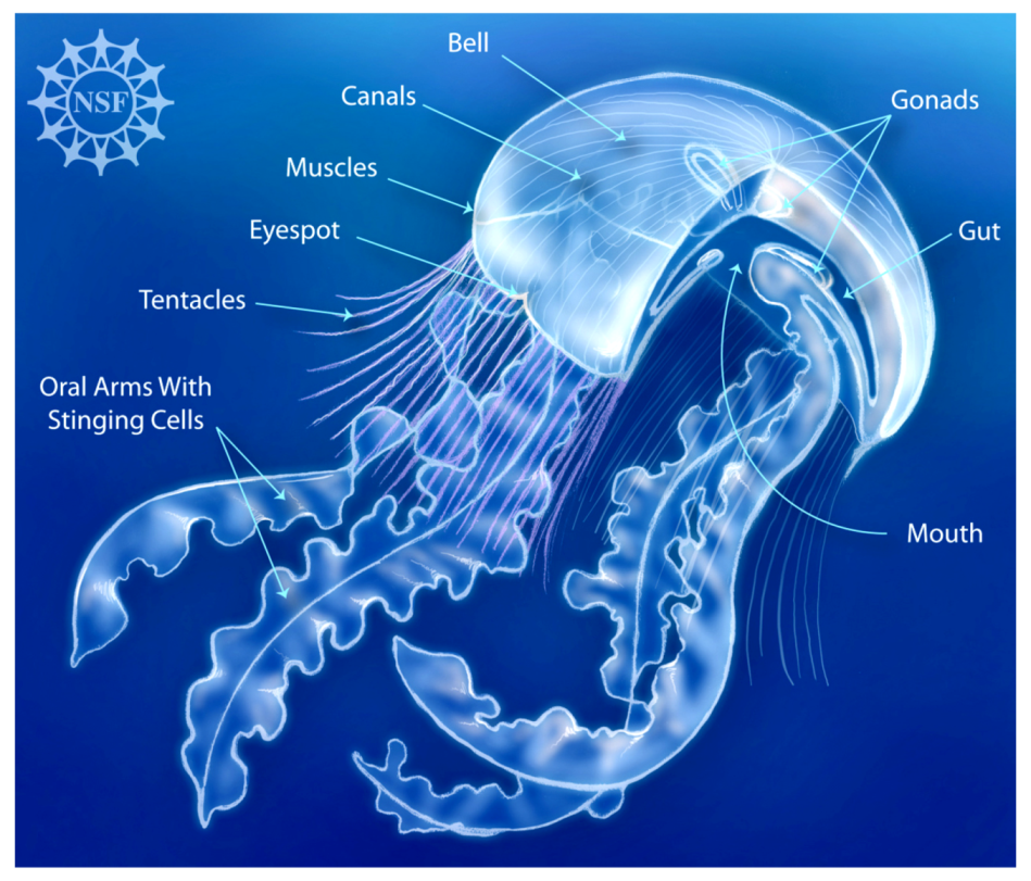
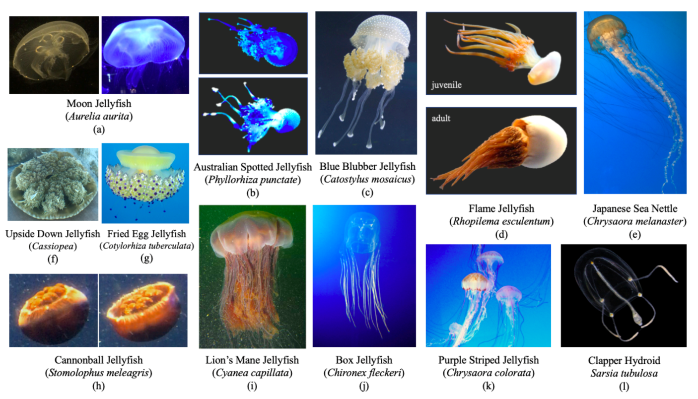
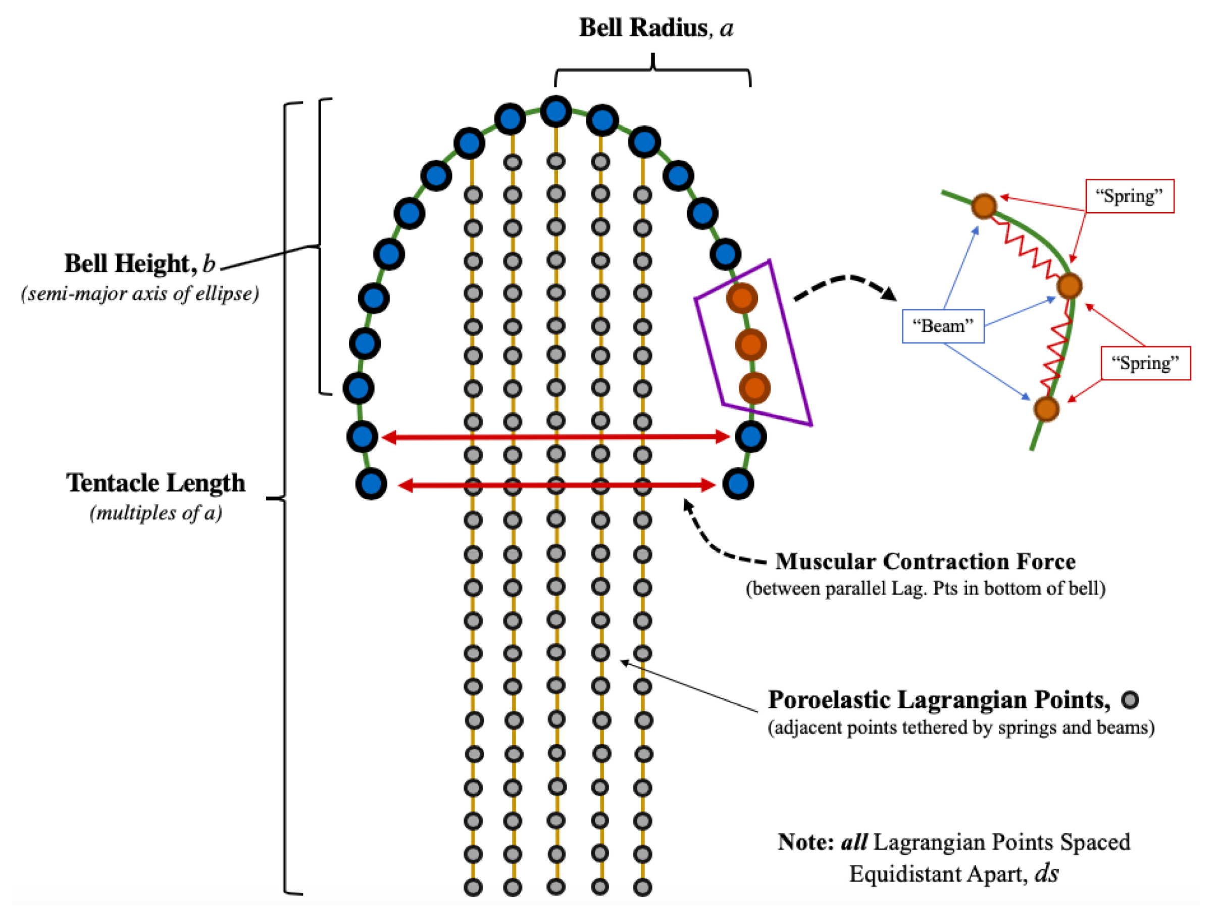
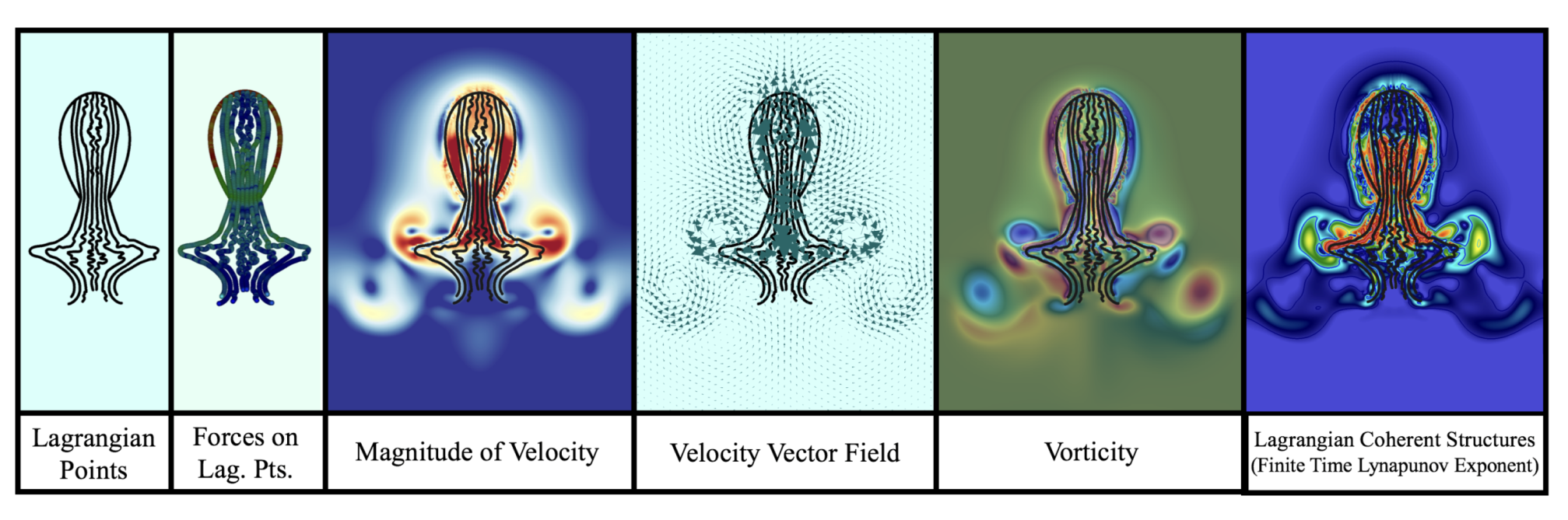
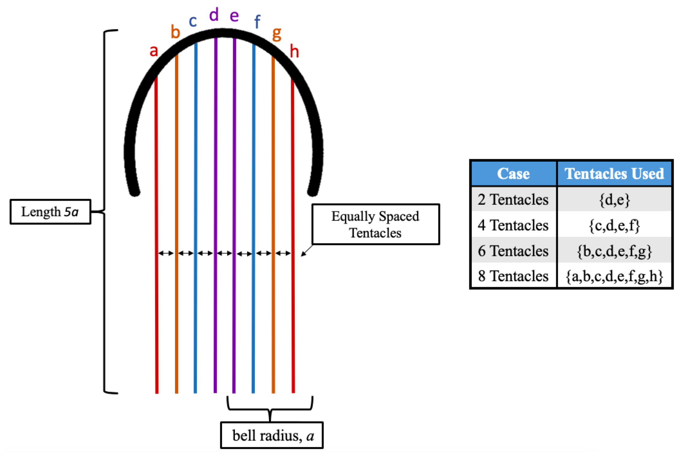
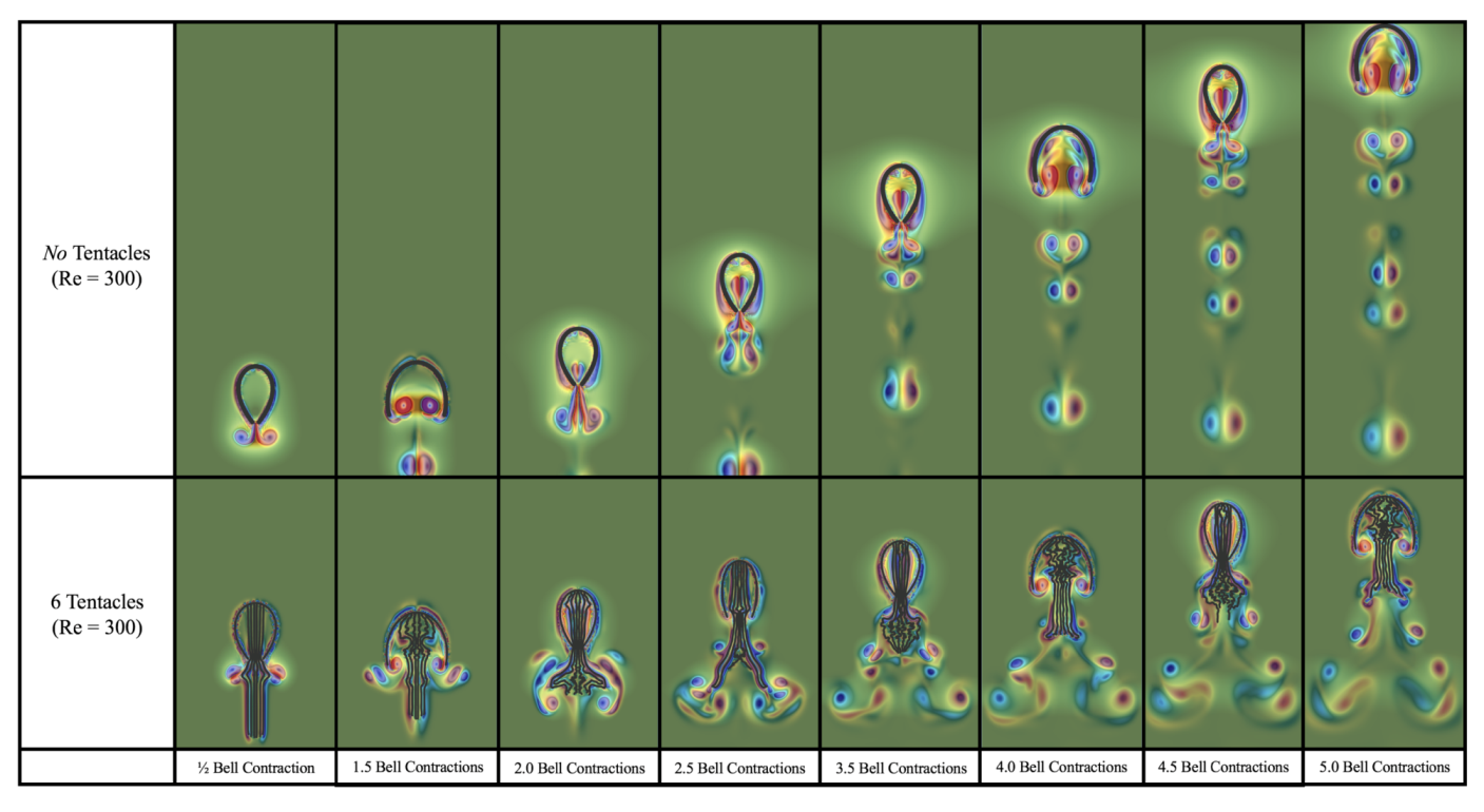
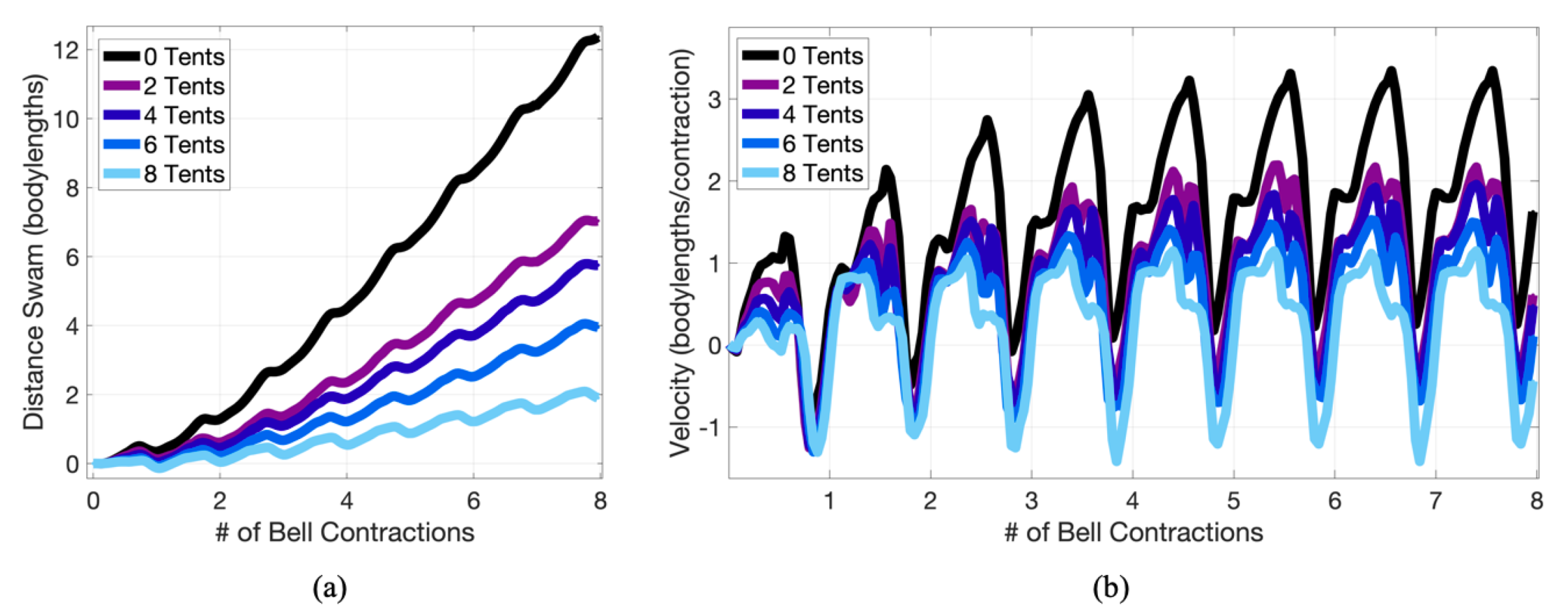
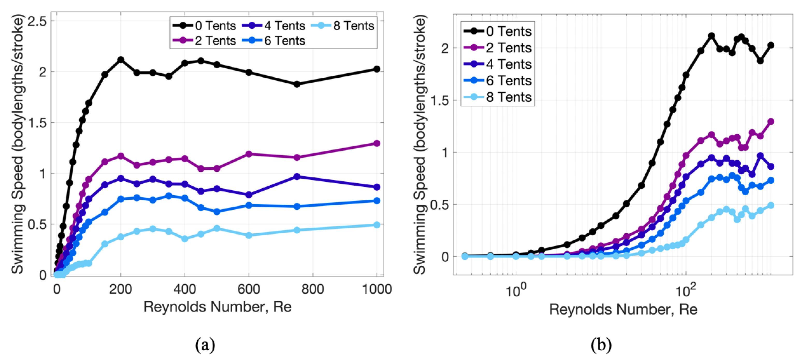
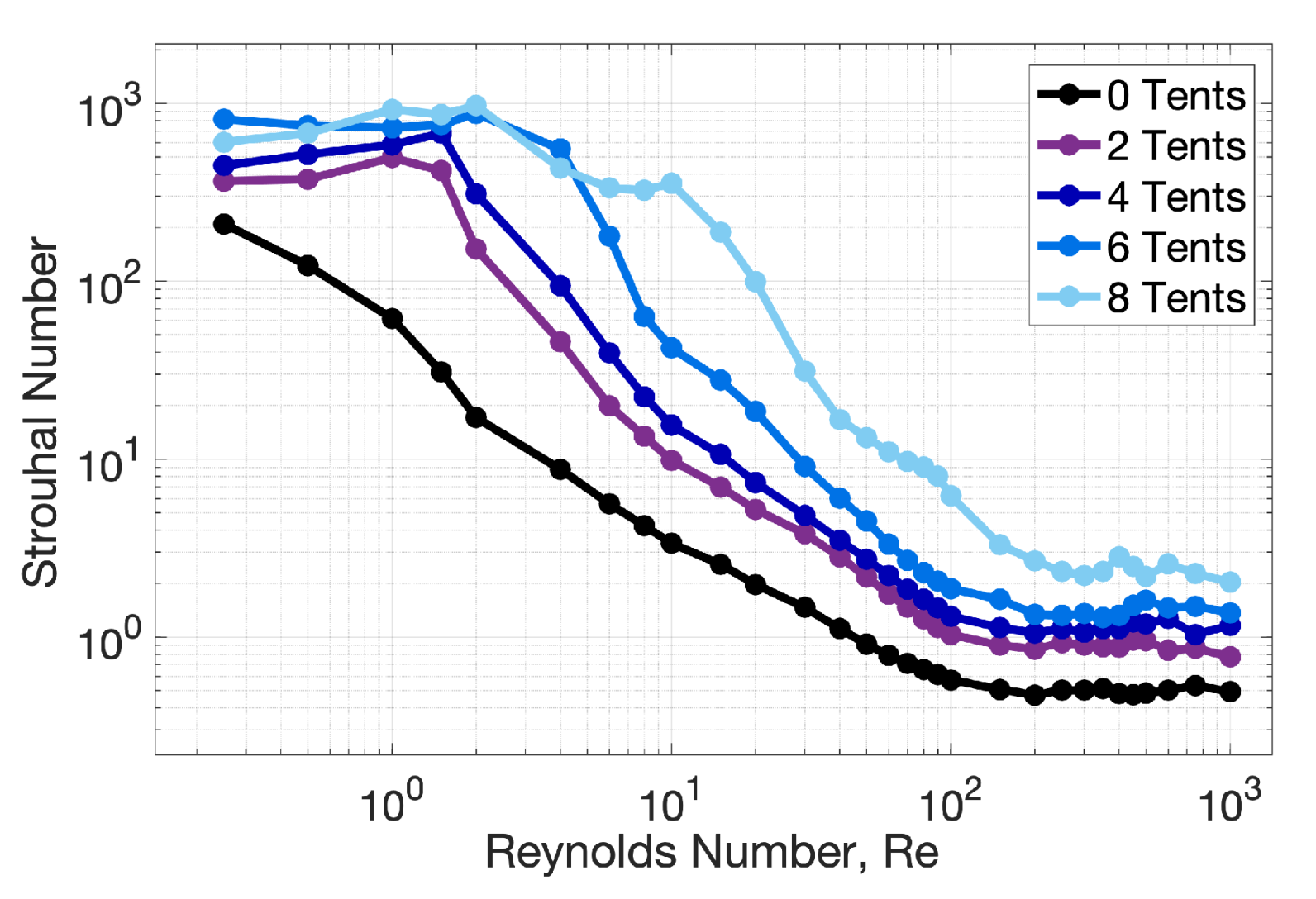
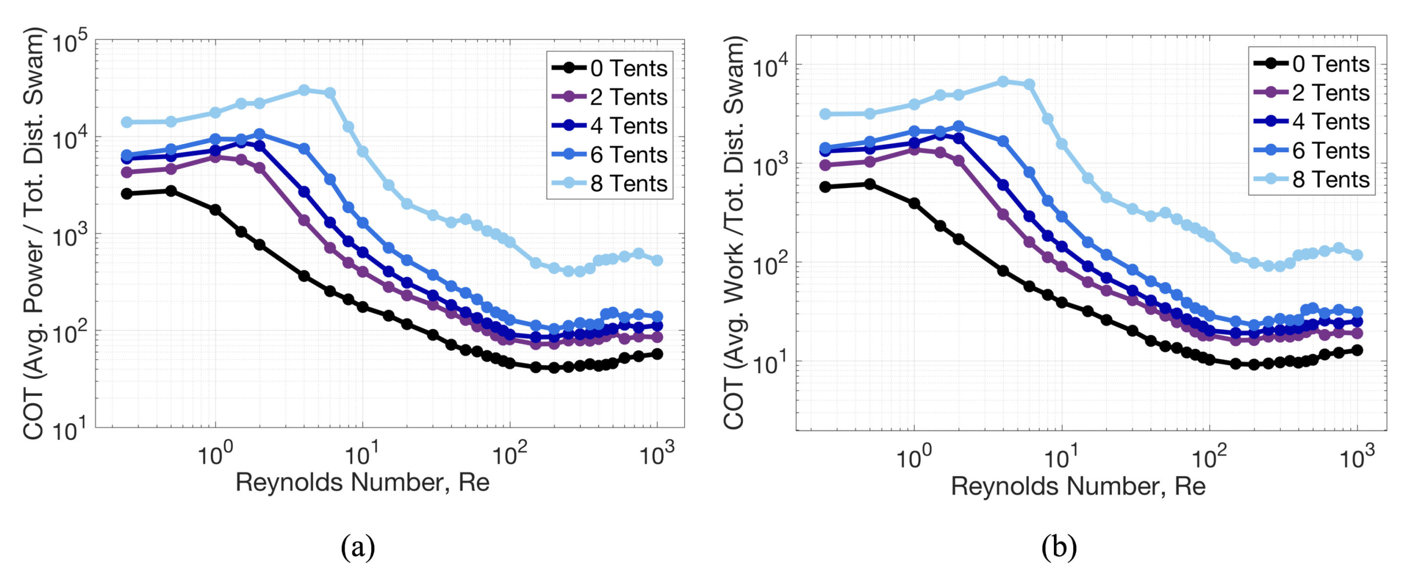
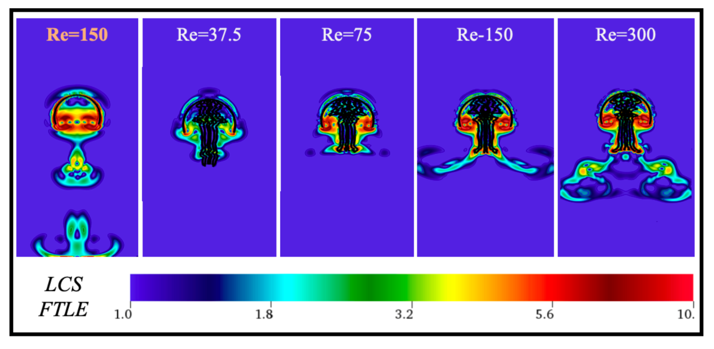
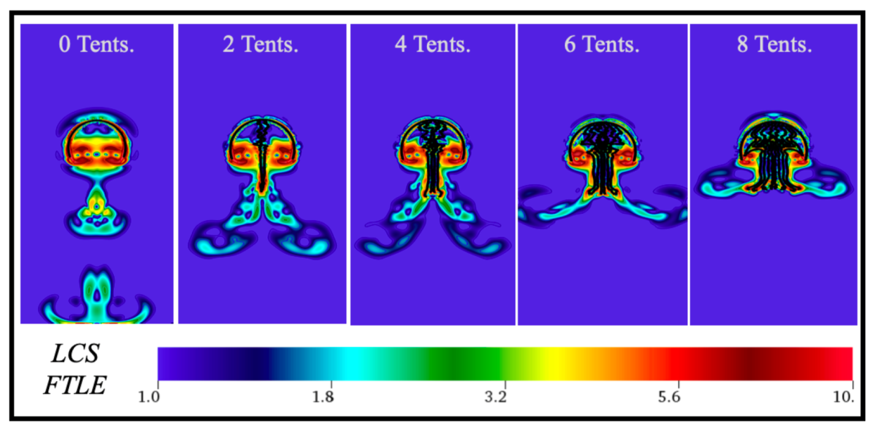
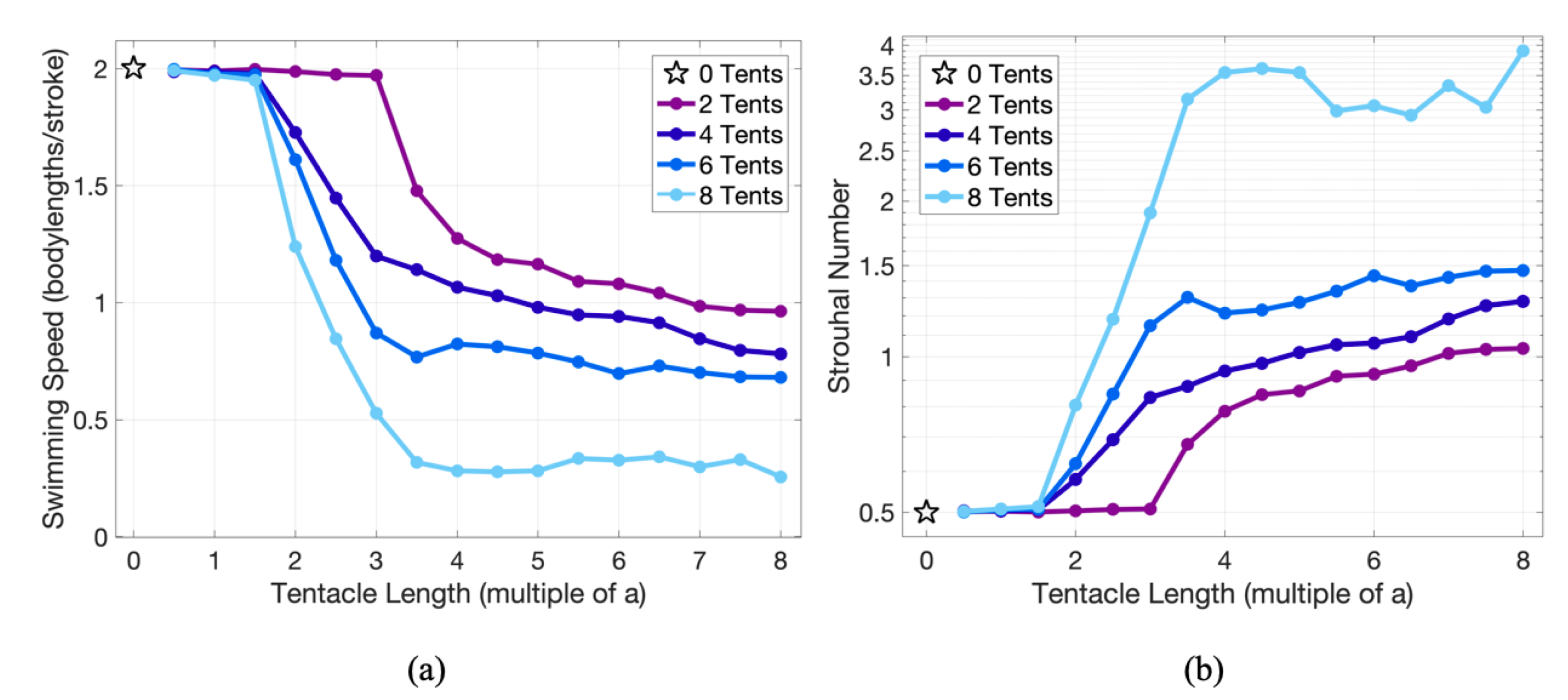
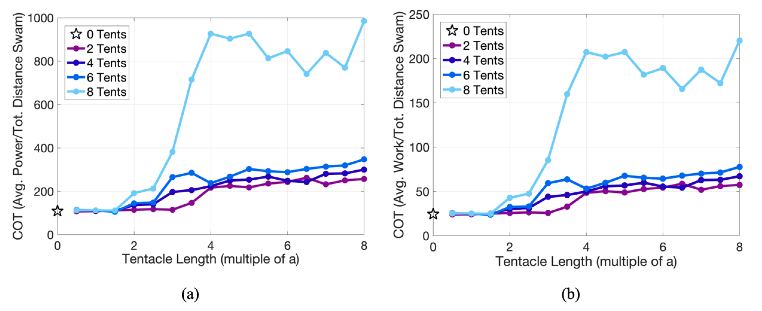
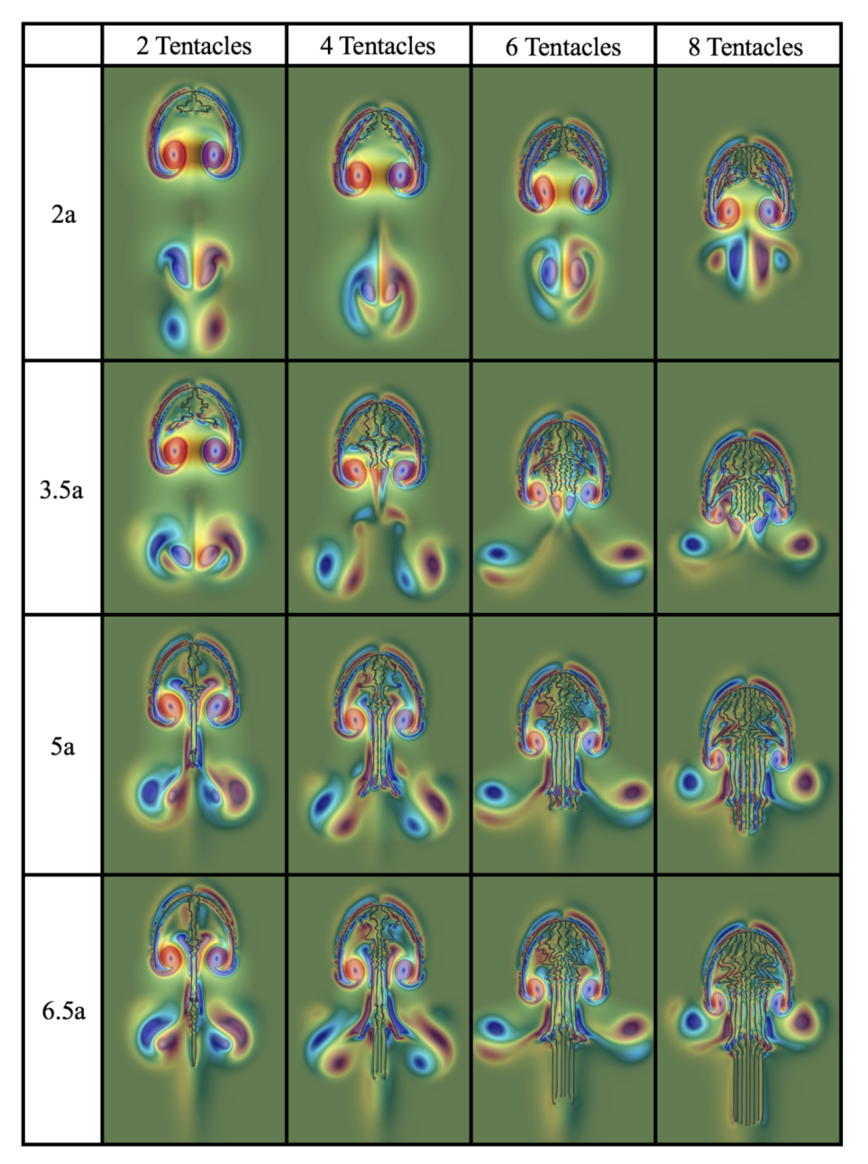
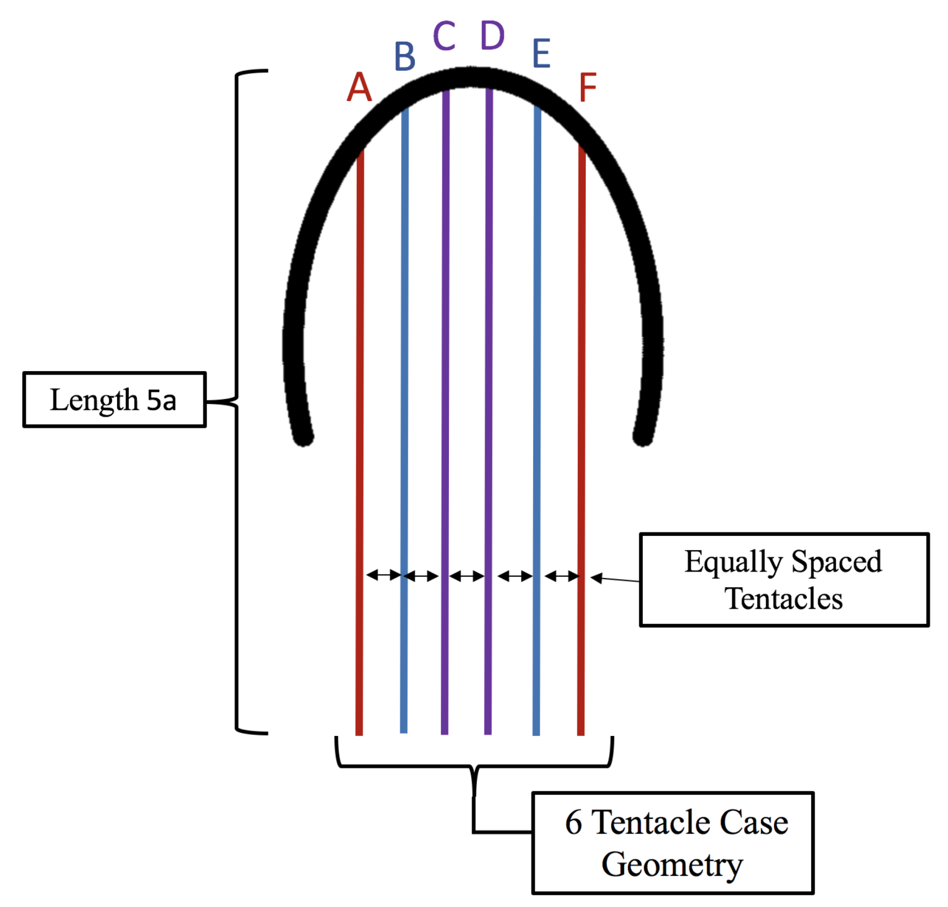
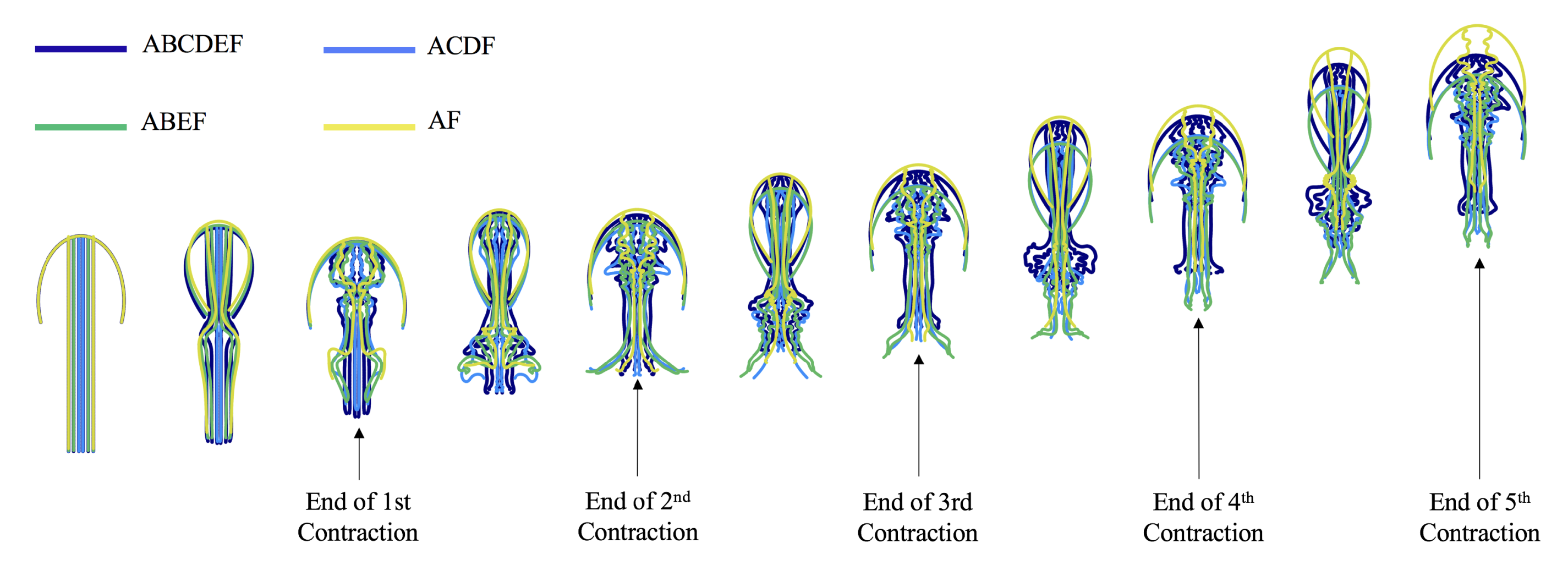
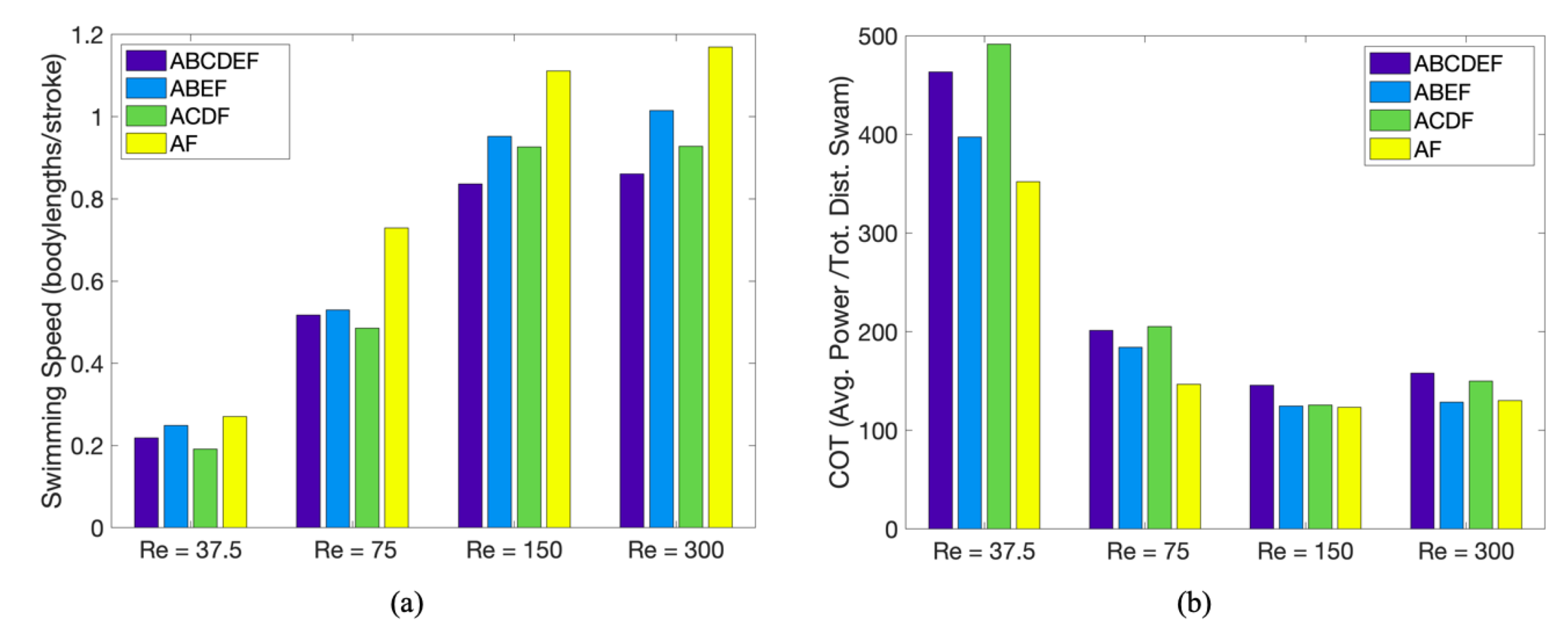
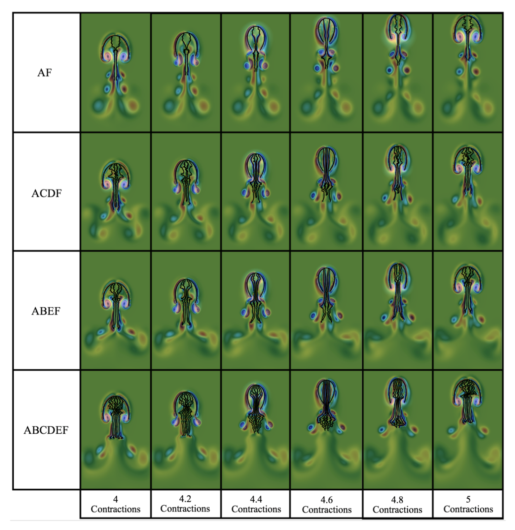
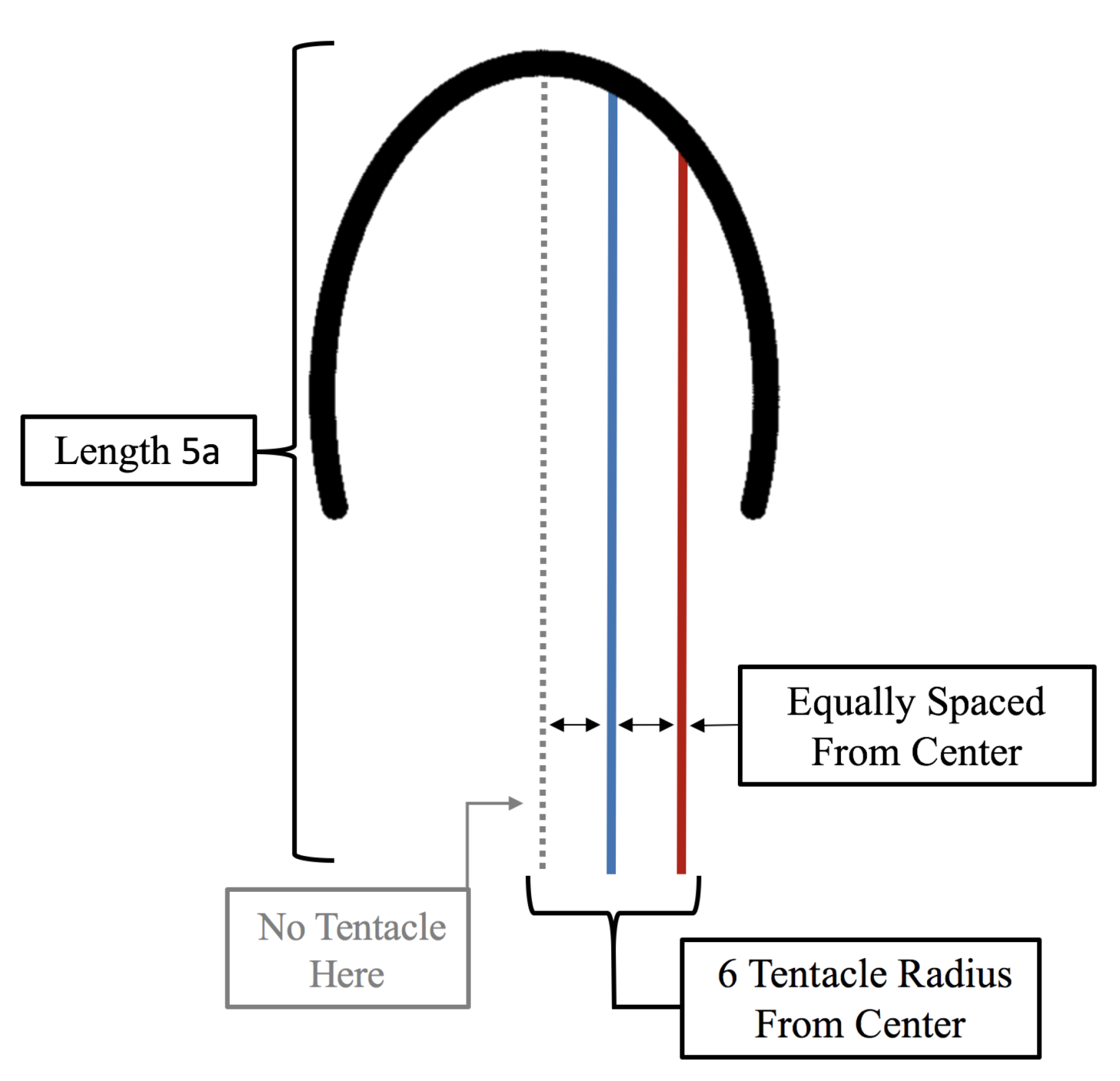
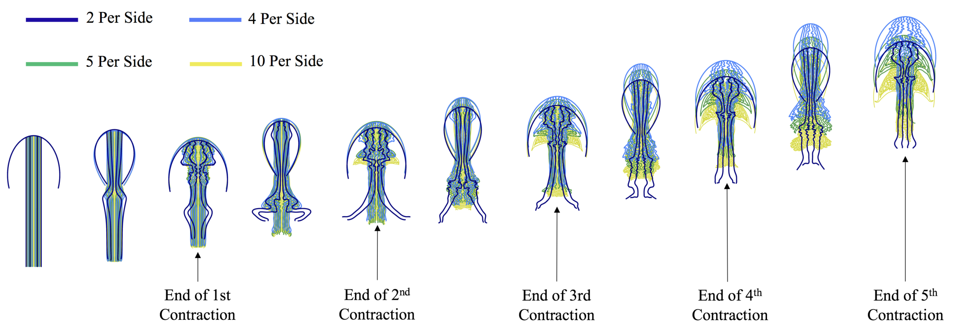
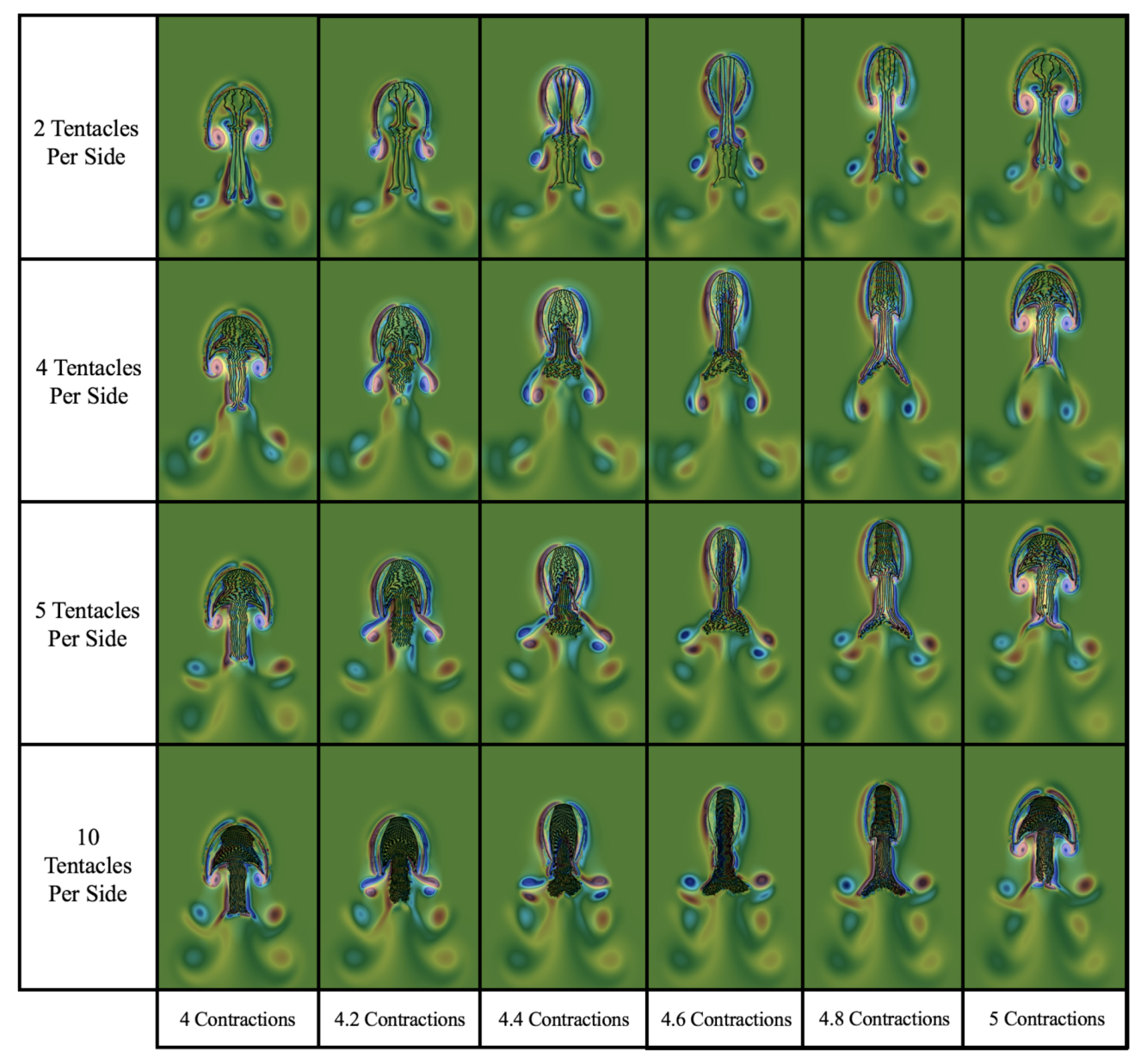
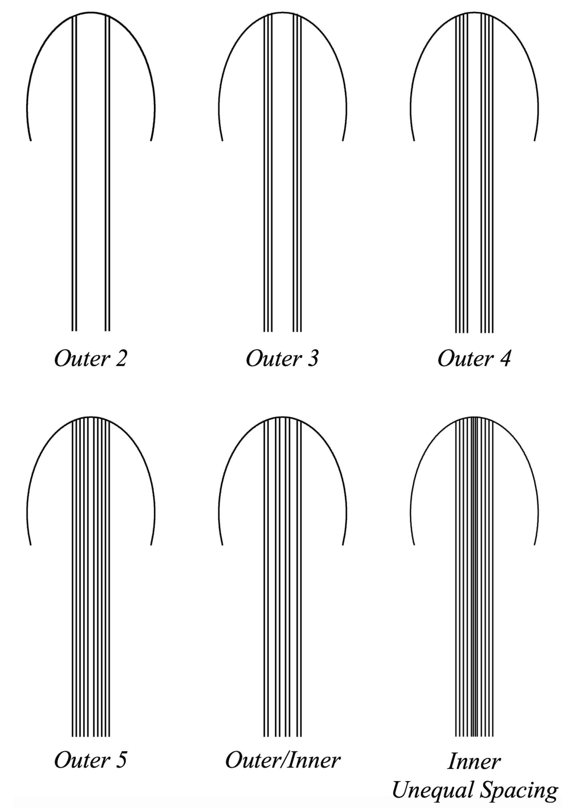
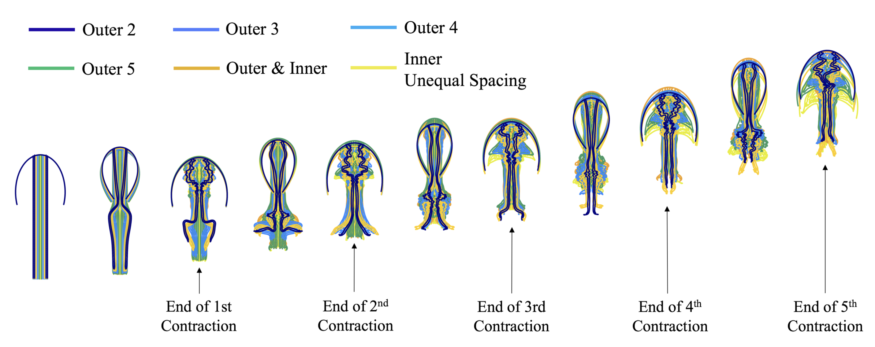
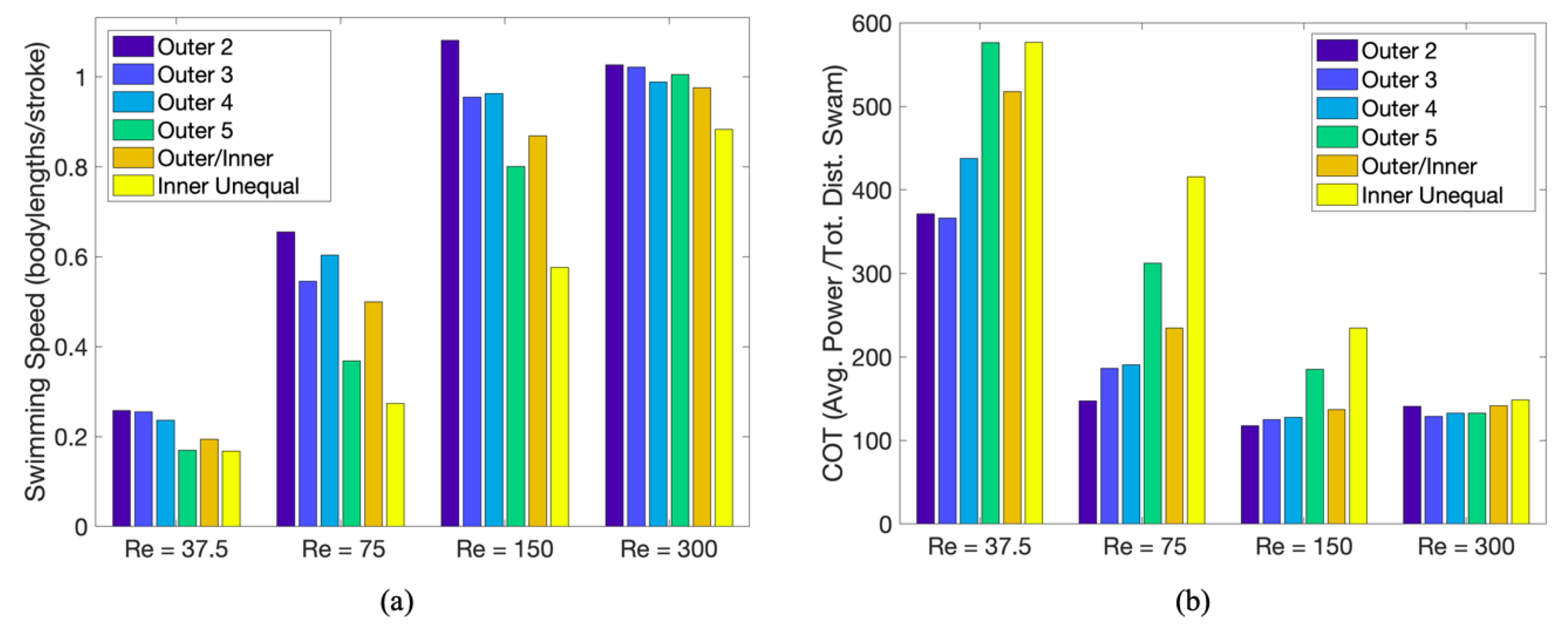
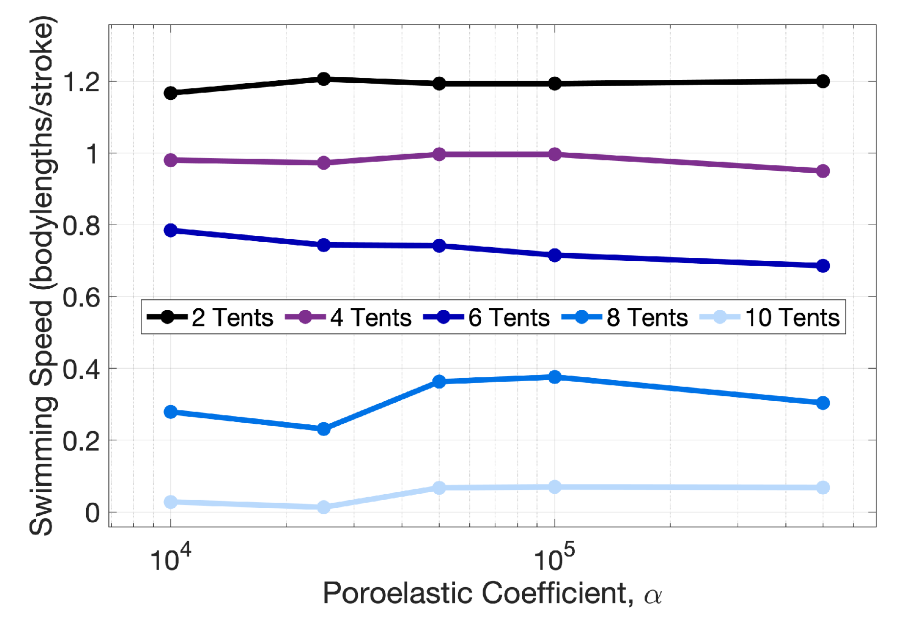
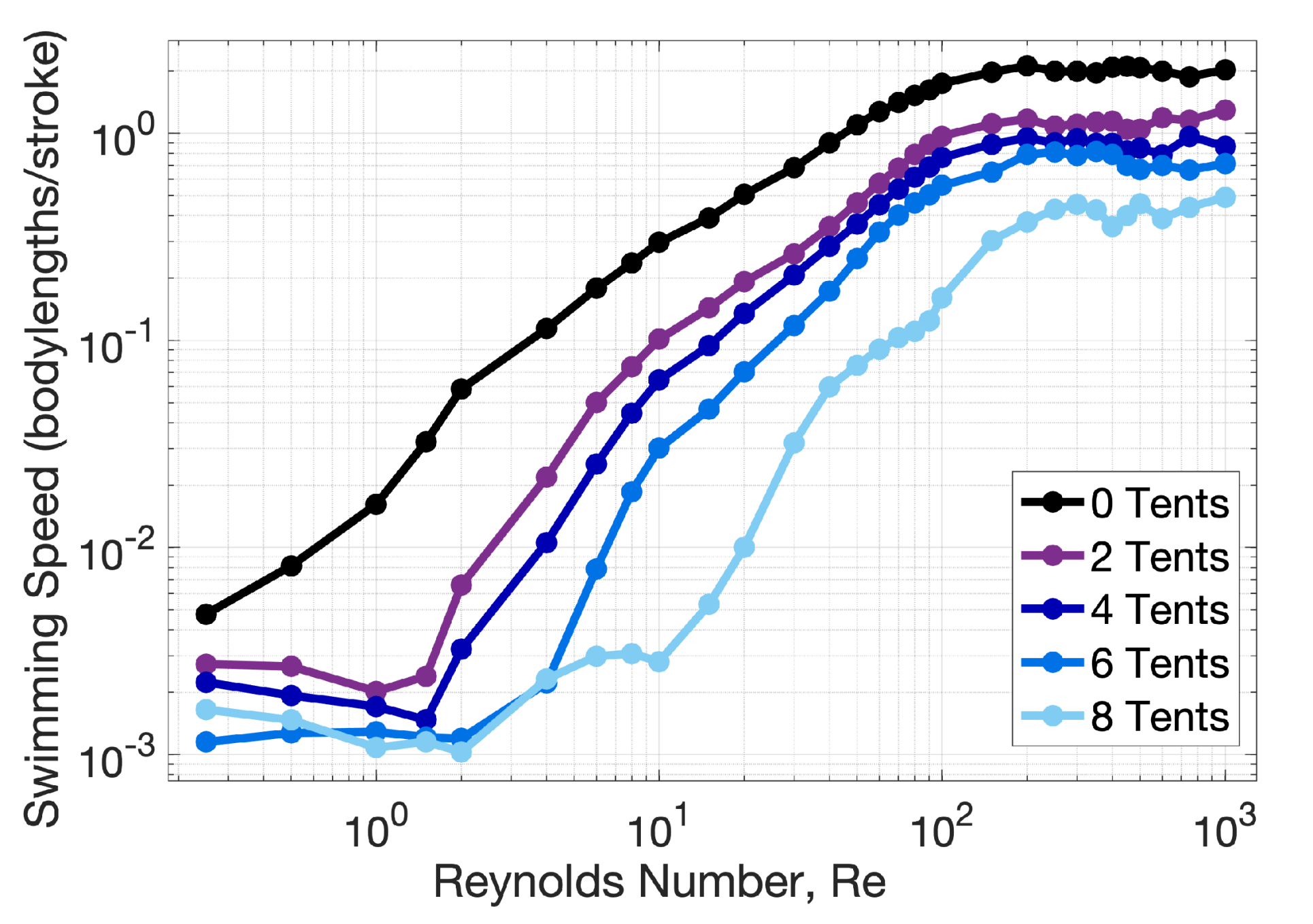
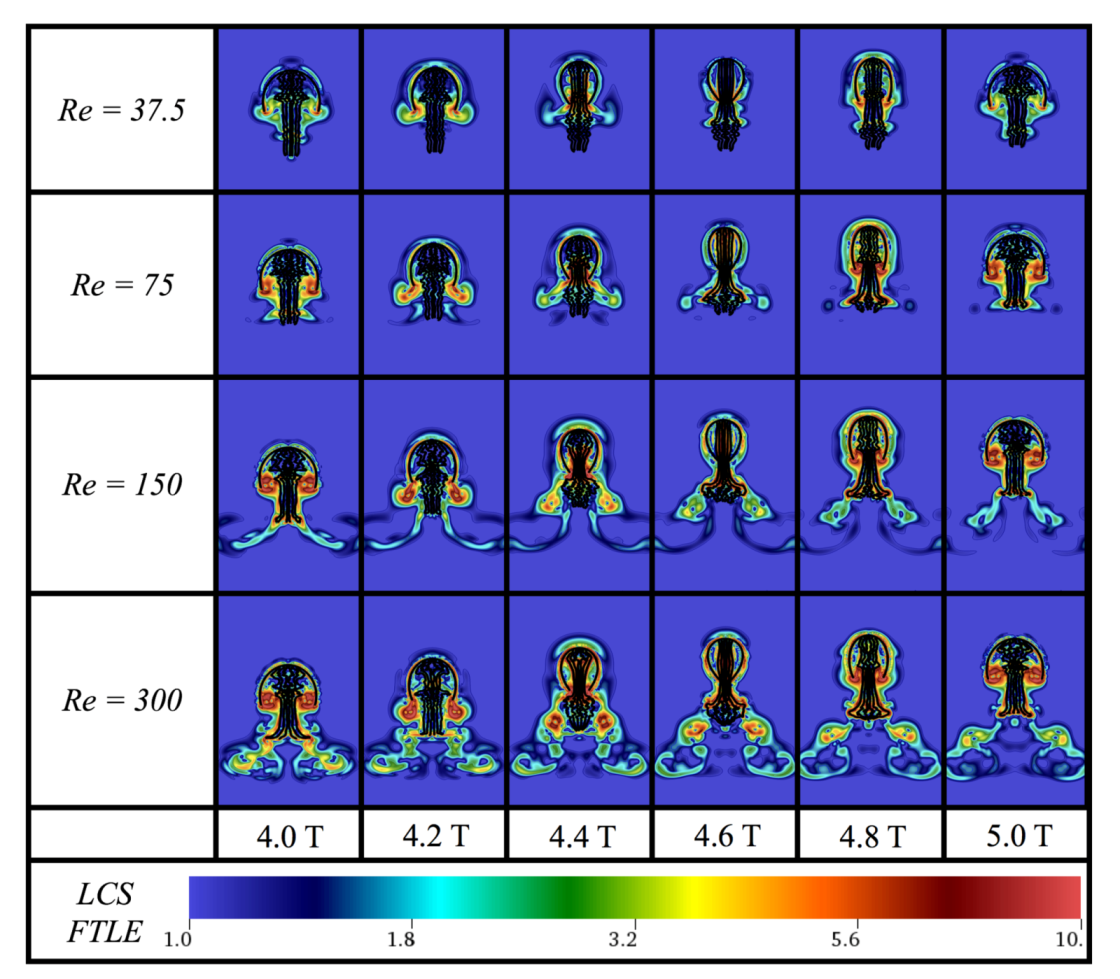
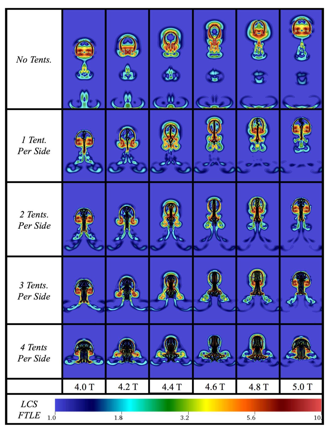
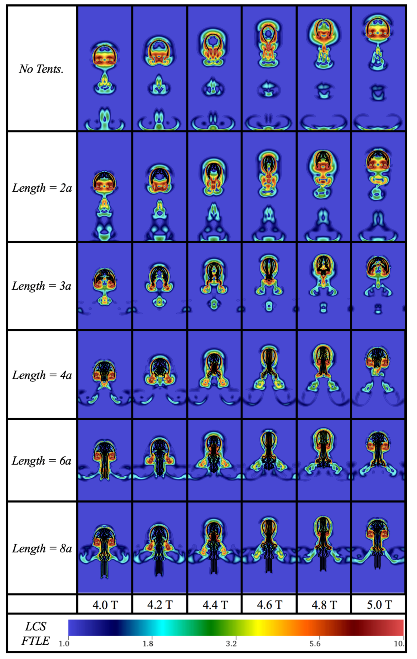
Table 1.
Morphological properties and range of the various jellyfish species shown in Figure 2.
Table 1.
Morphological properties and range of the various jellyfish species shown in Figure 2.
| Name | Scientific Name | Max. Bell Diameter (cm) | Tentacle/Oral Arm Length (cm) | Range | References |
|---|---|---|---|---|---|
| Moon Jellyfish | Aurelia aurita | 38 | Along the East & West Coast, Europe, Japan, and the Gulf of Mexico | [25] | |
| Australian Spotted Jellyfish | Phyllorhiza punctata | 60 | ≳60 | Western Pacific (From Australia to Japan) | [26,27] |
| Blue Blubber Jellyfish | Catostylus mosaicus | 45 | ∼45 | Along the east and north coasts of Australia | [28] |
| Flame Jellyfish | Rhopilema esculentum | 70 | ≳70 | Warm temperate waters of the Pacific Ocean | [27,29] |
| Japanese Sea Nettle | Chrysaora melanaster | 60 | 300 | Northern Pacific Ocean & adjacent parts of the Arctic Ocean | [30] |
| Upside-Down Jellyfish | Cassiopea | 36 | 36 | Western Atlantic, including the Gulf of Mexico, Bermuda, and the Caribbean | [31] |
| Fried Egg Jellyfish | Cotylorhiza tuberculata | 40 | ≳40 | Mediterranean Sea, coastal lagoons | [32] |
| Cannonball Jellyfish | Stomolophus meleagris | 25 | ≳25 | Pacific Ocean and the mid-west of the Atlantic Ocean | [33] |
| Lion’s Mane Jellyfish | Cyanea capillata | 250 | 3600 | Cold waters of the Arctic, Northern Atlantic, and Northern Pacific | [9,34] |
| Sea Wasp (Box Jellyfish) | Chironex fleckeri | 30 | 300 | Australia and Indo-West Pacific Ocean | [35,36] |
| Purple Striped Jellyfish | Chrysaora colorata | 70 | 800 | Eastern Pacific Ocean primarily off the coast of California | [37] |
| Clapper Hydroid | Sarsia tubulosa | 0.5 | 3–4 | Central California to the Bering Sea | [7,8] |
Table 2.
Numerical parameters used in the two-dimensional simulations.
| Parameter | Variable | Units | Value |
|---|---|---|---|
| Domain Size | m | ||
| Spatial Grid Size | m | ||
| Lagrangian Grid Size | m | ||
| Time Step Size | s | ||
| Total Simulation Time | T | pulses | 8 |
| Fluid Density | kg/m | 1000 | |
| Fluid Dynamic Viscosity | kg/(ms) | varied | |
| Bell Radius | a | m | (and varied) |
| Bell Diameter | D () | m | (and varied) |
| Bell Height | b | m | |
| Contraction Frequency | f | 1/s | |
| Spring Stiffness | kg·m/s | ||
| Beam Stiffness | kg·m/s | ||
| Tentacle Spring Stiffness | kg·m/s | ||
| Tentacle Beam Stiffness | kg·m/s | ||
| Muscle Spring Stiffness | kg·m/s | ||
| Poroelasticity Coefficient | m | varied |
Table 3.
Table giving the percentage difference in forward swimming speed when compared to the case with no tentacles/oral arms. Note that all cases with tentacles/oral arms are significantly slower.
Table 3.
Table giving the percentage difference in forward swimming speed when compared to the case with no tentacles/oral arms. Note that all cases with tentacles/oral arms are significantly slower.
| Total # Tentacles/Oral Arms | ||||
|---|---|---|---|---|
| 2 | −55.9% | −45.5% | −43.6% | −44.3% |
| 4 | −64.3% | −58.3% | −55.1% | −52.7% |
| 6 | −79.5% | −68.0% | −67.0% | −60.7% |
| 8 | −91.8% | −92.7% | −84.6% | −77.3% |
Table 4.
Table giving the percentage difference in forward swimming speed when compared to the case with no tentacles/oral arms. Note that all cases containing tentacles/oral arms are significantly slower.
Table 4.
Table giving the percentage difference in forward swimming speed when compared to the case with no tentacles/oral arms. Note that all cases containing tentacles/oral arms are significantly slower.
| ABCDEF | −71.1% | −64.1% | −57.4% | −57.6% |
| ABEF | −67.5% | −62.5% | −49.8% | −49.8% |
| ACDF | −74.7% | −65.5% | −51.1% | −52.6% |
| AF | −64.6% | −49.5% | −42.7% | −40.6% |
Table 5.
Table giving the percentage difference in forward swimming speed when compared to the case with no tentacles/oral arms. Note that all cases with tentacles/oral arms are significantly slower.
Table 5.
Table giving the percentage difference in forward swimming speed when compared to the case with no tentacles/oral arms. Note that all cases with tentacles/oral arms are significantly slower.
| 2 Per Side | −69.3% | −65.5% | −54.6% | −49.3% |
| 4 Per Side | −77.6% | −71.0% | −56.4% | −64.6% |
| 5 Per Side | −78.5% | −74.9% | −59.4% | −49.5% |
| 10 Per Side | −78.1% | −83.3% | −74.4% | −61.1% |
Table 6.
Table giving the percentage difference in forward swimming speed when compared to the case with no tentacles/oral arms. Note that all cases with tentacles/oral arms are significantly slower.
Table 6.
Table giving the percentage difference in forward swimming speed when compared to the case with no tentacles/oral arms. Note that all cases with tentacles/oral arms are significantly slower.
| Outer 2 | −67.4% | −55.3% | −45.2% | −48.4% |
| Outer 3 | −67.7% | −62.7% | −51.6% | −48.6% |
| Outer 4 | −70.1% | −58.8% | −51.2% | −50.3% |
| Outer 5 | −78.5% | −74.9% | −59.4% | −49.5% |
| Outer/Inner | −75.4% | −65.9% | −55.9% | −51.0% |
| Inner Unequal | −78.8% | −81.3% | −70.8% | −55.6% |
© 2019 by the authors. Licensee MDPI, Basel, Switzerland. This article is an open access article distributed under the terms and conditions of the Creative Commons Attribution (CC BY) license (http://creativecommons.org/licenses/by/4.0/).
Share and Cite
MDPI and ACS Style
Miles, J.G.; Battista, N.A. Naut Your Everyday Jellyfish Model: Exploring How Tentacles and Oral Arms Impact Locomotion. Fluids 2019, 4, 169. https://doi.org/10.3390/fluids4030169
AMA Style
Miles JG, Battista NA. Naut Your Everyday Jellyfish Model: Exploring How Tentacles and Oral Arms Impact Locomotion. Fluids. 2019; 4(3):169. https://doi.org/10.3390/fluids4030169
Chicago/Turabian StyleMiles, Jason G., and Nicholas A. Battista. 2019. "Naut Your Everyday Jellyfish Model: Exploring How Tentacles and Oral Arms Impact Locomotion" Fluids 4, no. 3: 169. https://doi.org/10.3390/fluids4030169