Cervical Cancer Diagnostics Using Machine Learning Algorithms and Class Balancing Techniques

Abstract

Objectives: Cervical cancer is present in most cases of squamous cell carcinoma. In most cases, it is the result of an infection with human papillomavirus or adenocarcinoma. This type of cancer is the third most common cancer of the female reproductive organs. The risk groups for cervical cancer are mostly younger women who frequently change partners, have early sexual intercourse, are infected with human papillomavirus (HPV), and who are nicotine addicts. In most cases, the cancer is asymptomatic until it has progressed to the later stages. Cervical cancer screening rates are low, especially in developing countries and in some minority groups. Due to these facts, the introduction of a tentative cervical cancer screening based on a questionnaire can enable more diagnoses of cervical cancer in the initial stages of the disease. Methods: In this research, publicly available cervical cancer data collected on 859 female patients are used. Each sample consists of 36 input attributes and four different outputs Hinselmann, Schiller, cytology, and biopsy. Due to the significant unbalance of the data set, class balancing techniques were used, and these are the Synthetic Minority Oversampling Technique, the ADAptive SYNthetic algorithm (ADASYN), SMOTEEN, random oversampling, and SMOTETOMEK. To obtain the mentioned target outputs, multiple artificial intelligence (AI) and machine learning (ML) methods are proposed. In this research, multiple classification algorithms such as logistic regression, multilayer perceptron (MLP), support vector machine (SVM), K-nearest neighbors (KNN), and several naive Bayes methods were used. Results: From the achieved results, it can be seen that the highest performances were achieved if MLP and KNN are used in combination with Random oversampling, SMOTEEN, and SMOTETOMEK. Such an approach has resulted in mean area under the receiver operating characteristic curve ($\overline{AUC}$) and mean Matthew’s correlation coefficient ($\overline{MCC}$) scores of higher than $0.95$, regardless of which diagnostic method was used for output vector construction. Conclusions: According to the presented results, it can be concluded that there is a possibility for the utilization of artificial intelligence (AI) and machine learning (ML) techniques for the development of a tentative cervical cancer screening method, which is based on a questionnaire and an AI-based algorithm. Furthermore, it can be concluded that by using class balancing techniques, a certain performance boost can be achieved.

1. Introduction

In this section, a brief introduction to the problem of cervical cancer screening rates and the application of artificial intelligence (AI) methods for tentative cervical cancer diagnosis will be provided. Furthermore, the state-of-the-art will be presented.

1.1. General Information about Cervical Cancer

Cervical cancer ranks fourth among malignant diseases in women, right after breast cancer, colon cancer, and lung cancer. In Europe, the incidence of cervical cancer ranges from 12–30 per 100,000 women. In almost all countries of the world, a constant decrease in the frequency of cervical cancer has been recorded in recent years, which is primarily due to an improved early diagnosis of pre-stages and the changes that precede them. In earlier years, cervical cancer accounted for up to 70% of all genital cancers, while today, the frequency is around 35–50% with a tendency of further decrease. It most often occurs in women between the ages of 20 and 40, with the decline in incidence being more visible in women over 40, with 1–2% of women in that age group having cervical cancer [1,2,3]. Cervical cancer occurs when the cells of the cervix, the lower part of the uterus, undergo abnormal changes and create precancerous cells that gradually turn into cancer cells. In 90–95% of cases, cervical cancer develops relatively slowly, over a period of 5 to 10 years, and is preceded by several pre-stages or stages of dysplasia (CIN I, CIN II, and CIN III), while only in 5–10% of cases, cancer can occur without any signs and earlier changes in screening tests. Given that the disease develops over a period of several years, a systematic gynecological examination enables the detection of the disease at an early stage when the disease is completely curable. The immediate precursors of cancer are severe dysplasia (CIN III–cervical intraepithelial neoplasia of the third degree), or carcinoma in situ (CIS), and they are usually preceded by mild dysplasia (CIN I) and moderate dysplasia (CIN II) changes for a long period [1,4]. Cervical cancer treatment usually includes surgical resection, radiation, and chemotherapy. Healing and prognosis depend on the stage of cancer and the treatment measures taken [5].

1.2. Cervical Cancer Diagnosis

Given that changes from normal cervical mucus to clinically clearly visible cancer in most cases develop over a period of several years, regular gynecological examination, PAPA test, colposcopy, and HPV typing give us enough time to detect these changes promptly, treat them adequately, and completely prevent the occurrence of cervical cancer. There are two main types of cervical cancer: squamous cell cancer (70–80%), and adenocarcinoma, which develops from glandular cells that produce mucus that lines the cervical canal. Adenocarcinoma is less common than squamous cell carcinoma, but in recent years, it has become more common and it now accounts for 10 to $15\%$ of uterine cancers. Since adenocarcinoma arises in the cervical canal and not in the cervix itself, it is more difficult to detect through screening than squamous cell cancer of the cervix, but the treatment is the same [6,7]. Cervical cancer is caused by certain types of human papillomavirus (HPV), and the main causative agents are high-risk types of HPV. It is important to emphasize that there are risk factors that can increase the risk of developing cervical cancer in women infected with HPV. Some of the risk factors are: smoking, early sexual intercourse, promiscuity, infection with genital herpes, immunosuppression, lower socioeconomic status, poor genital hygiene, and a higher number of births [8,9]. Symptoms depend on the extent of the tumor and the stage of the disease, but the problem arises in the pre-stage of cancer because it is usually asymptomatic. Changes in the cervix are usually discovered by chance during regular annual check-ups. Advanced stages show clear symptoms in about 90% of cases. Irregular bleeding is the main symptom of cervical cancer. It occurs as:

• spotting,
• brownish discharge,
• postmenopausal bleeding, or
• contact bleeding (bleeding during sexual intercourse or defecation).

Another important symptom is the appearance of bloody discharge, usually with an unpleasant smell. In addition to these symptoms, pain in the lower abdomen can occur, usually in advanced stages of the disease, with the involvement of neighboring organs [10].

1.3. Cervical Cancer Screening Rates

It can be seen that a certain form of gynecological examination is performed during cervical cancer screening. Such a diagnostic procedure can be painful [11,12] and unpleasant [13] for a patient. The unpleasant nature of gynecological examination can cause delay and avoidance [14], which can prevent early diagnosis. Furthermore, a lack of proper public health policies in developing countries can cause low cervical cancer screening rates. Such circumstances are responsible for 18 times higher mortality [15]. In 9 out of 10 cervical, cancer-related deaths occur in low-income countries [16]. Due to the fact that early-stage cervical cancers have promising survival rates that can achieve $90\%$ in a 5-year period [17], an increase in cervical cancer screening rates presents an absolute imperative. Cervical cancer screening rates are different for different countries, ranging from high in developed countries [18] to extremely low in developing countries. In the next few paragraphs, a brief overview of cervical cancer screening rates is presented. The authors in [19] have analyzed the data collected from women living in Olmsted County, Minnesota. The study was performed on data for each year from 2005 (47,203 women) to 2016 (49,510 women). The results show that in 2016, $64.5\%$ of women between 30 and 65 were regular with cervical cancer screenings. Furthermore, $60.8\%$ of women have performed combined Papanicolau (Pap) and HPV tests. The authors in [20] have performed a study that uses data from commercial insurance companies in the United States from 2003 to 2014. From the presented results it can be seen that less than $5\%$ of women between 18 and 20 years of age are attending regular cervical cancer screenings. For women between 21 and 29, the number is around $16\%$. The highest rate of cervical cancer screening is in the age group between 30 and 39, where $44\%$ of women attend regular cervical cancer screenings. For the age group 40–49 and 50–65 the rates are 38% and 28%, respectively. The rates of cervical cancer screening are significantly influenced by socio-economic circumstances, as well as ethnicity [2]. The authors in [21] have shown that women with unstable socio-economic backgrounds tend to skip PAP test. The lowest rate of Pap test can be noticed for the case of women without a usual source of healthcare and uninsured women, with rates of $65.1\%$ and $63.8\%$, respectively. Furthermore, the study has shown that Asian ($75.8\%$) and Hispanic ($78.6\%$) women have lower cervical cancer screening rates than non-Hispanic White ($83.7\%$) and Black women ($85.3\%$). The low rate of cervical cancer and HPV screening can be particularly emphasized in middle and low-income countries. From the study presented in [22], it can be seen that the highest rate of cervical cancer screenings in middle- and low-income countries is achieved in the Caribien area and Latin America (median $84.6\%$). The lowest rates of cervical cancer screenings are achieved in sub-Saharan Africa with a median of $16.9\%$.

1.4. Survey-Based Cervical Cancer Diagnostics

For these reasons, and with the aim of increasing the rate of women included in cervical cancer screening, an approach based on an online survey is proposed. By using such an approach, a tentative evaluation and cervical cancer forecasting can be achieved without the need for standard cervical cancer screening, which can often be unpleasant and inaccessible for a large part of the female population. The original research for such an approach was published in [23], where the authors have proposed a data set that consists of 32 input parameters and four output parameters, the diagnostics collected by using Biopsy, Cytology, Hinselmann evaluation, and Shiller evaluation. A brief overview of the different research papers and the achieved results is presented in

Table 1. A brief overview of the state-of-the-art methods and results ($TPR$—true positive rate, $TNR$—true negative rate, $Acc$—Accuracy, $F1$—$F1$-score).

Article	Method	Biopsy	Cytology	Hinselmann	Shiller
[24]	RF + SMOTE	$TPR$ = $0.93$; $TNR$ = $0.98$	$TPR$ = $0.98$; $TNR$ = $0.99$	$TPR$ = $0.96$; $TNR$ = $0.98$	$TPR$ = $0.93$; $TNR$ = $0.98$
[25]	Autoencoder	$Acc=0.96$	$Acc=0.97$	$Acc=0.97$	$Acc=0.96$
[26]	XGBoost	$F1=0.96$	$F1=0.94$	$Acc=0.98$	$Acc=0.96$
[27]	RF	$Acc=0.98$	$Acc=0.98$	$Acc=0.99$	$Acc=0.98$
[28]	RF + SMOTE	$TPR$ = $0.97$; $TNR$ = $0.97$	$TPR$ = $0.98$; $TNR$ = $0.98$	$TPR$ = $0.96$; $TNR$ = $0.95$	$TPR$ = $0.97$; $TNR$ = $0.97$

.

From the literature overview, two main research gaps can be noticed:

1

There is no detailed analysis about the utilization of more complex class balancing techniques instead of SMOTE.

2

There is no analysis of the classification performances of different combinations of class balancing techniques and ML classifiers.

It can be seen that the methods presented in state-of-the-art have often low classification performances. Furthermore, it can be noticed that a certain number of the research is evaluated by using inappropriate validation measures such as Accuracy.

1.5. Research Hypotheses

According to the presented literature overview and by using the identified research gap, the following questions can be asked:

• Is it possible to apply data balancing techniques to increase the classification performances of ML classifiers for cervical cancer diagnosis?
• How does the combination of the class balancing technique and ML classifier influence the classification performances?
• How does the combination of the class balancing technique and ML classifier influence the generalization performances?
• Is it possible to use developed methods for tentative cervical cancer screening?

The novelty of this paper can be divided into two main parts. The first main novelty is the definition of the algorithmic foundation for the development of an online tool for questionnaire-based cervical cancer screening. The presented method is intended for the public health system, where the application of AI algorithms will provide initial cervical cancer screening, based on a questionnaire. For this research, a publicly available data set is used for the investigation of given hypotheses. The collection of new data set is defined as one of the future investigations. The second main novelty is the examination of the different combinations of class balancing techniques and ML-based classification algorithms. The determined combinations will be used to develop a questionnaire-based cervical cancer survey.

This paper is divided into seven sections. In the Section 2, a comparison of standard diagnostic procedures and tentative AI-based screening is presented. Section 3 is dedicated to the data set description and the description of class balancing techniques that are used in this research. In the Section 4 and Section 5, a brief description of ML classifiers used is provided, followed by a detailed overview of the research methodology. Section 6 and Section 7 are dedicated to the results, discussion, and conclusions.

2. Standard Cervical Cancer Diagnostic Procedure and AI-Based Tentative Screening

In this section, a brief description of standard cervical cancer screening methods and diagnostic methods is provided. The standard screening methods are compared with the results of state-of-the-art AI-based screening methods. In the end, a description of the proposed AI-based tentative screening is provided.

2.1. Standard Cervical Cancer Screening and Colposcopy

The initial step in the diagnosis of cervical cancer is based on several screening methods, of which the most common are:

• Papanicolaou (PAP) test,
• Liquid-Based Cytology (LBC),
• HPV-DNA testing.

A PAP test is a cytological method in which the gynecologist uses a wooden spatula and a wooden stick wrapped in cotton wool to take a swab from the posterior arch of the cervix, the cervical part of the cervix, and the cervical canal. The swab is transferred from a wooden spatula and stick to a glass slide that is immersed in alcohol to fix (preserve) the cells, and is stained using a special method so that the taken cells can be analyzed microscopically [29]. LBC is a cytological analysis performed to detect the changes that precede cervical cancer. The main difference between LBC and PAP is the application of the cells to the glass using a conservation solution. Such a sample is more suitable for analysis because it does not contain blood, mucus, and inflammatory cells [30]. HPV-DNA is a diagnostic method where the cervix is visualized with a speculum, and a sample is taken from the cervical canal with a swab that has a cotton head or a brush, and delivered to the laboratory in a transport medium. The sample’s DNA is analyzed to determine if the patient has been infected with an HPV type that correlates with cervical cancer occurrence [31].

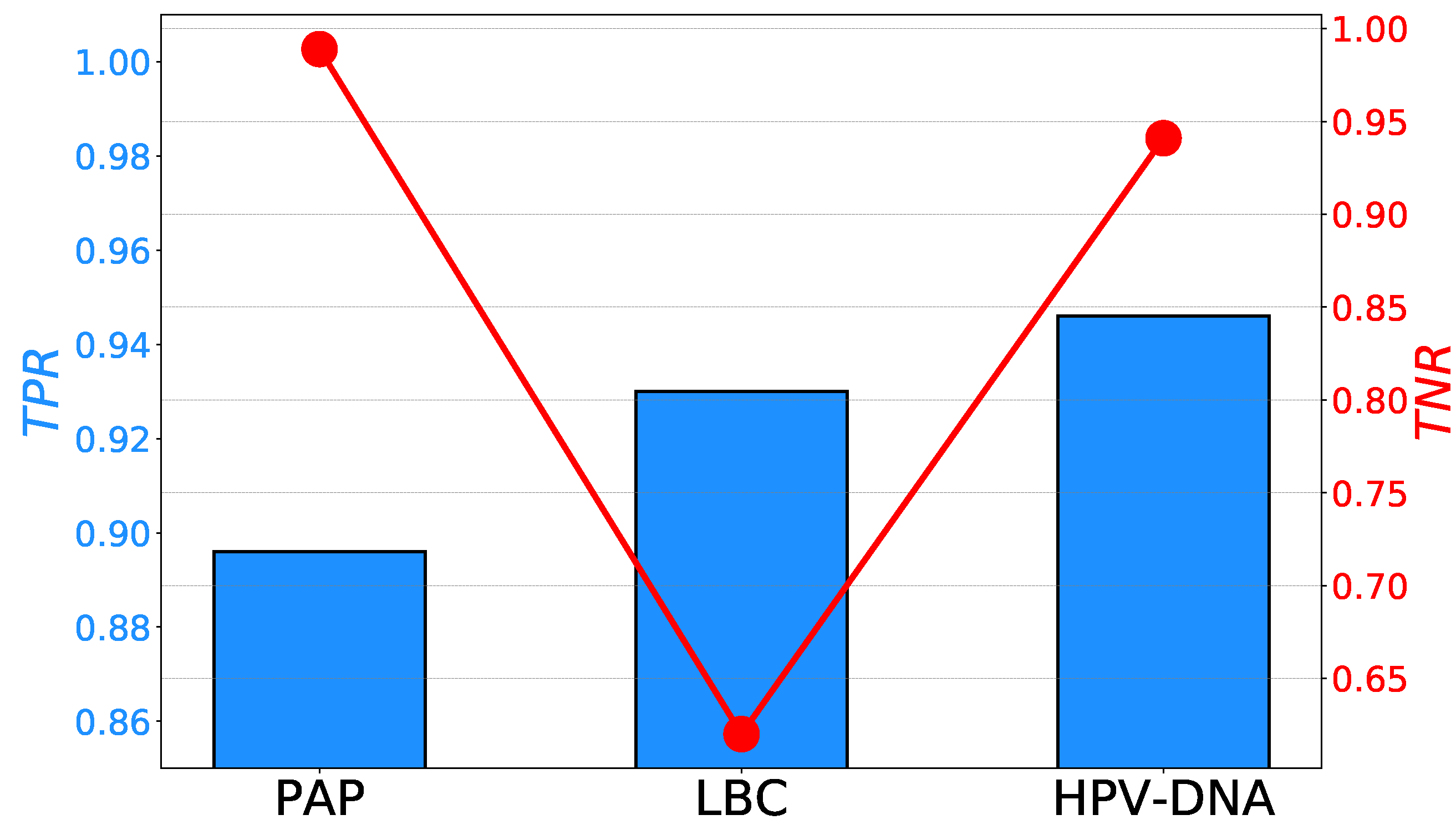
The $TPR$ and $TNR$ rates achieved with PAP, LBC, and HPV-DNA methods are reported in multiple research and review papers [32,33,34,35]. The comparison of maximal $TPR$ and $TNR$ rates are presented in Figure 1. If the $TPR$ and $TNR$ rates achieved with PAP, LBC, and HPV-DNA are compared with state-of-the-art survey-based methods presented in Table 1, and it can be seen that survey-based methods are achieving similar and even higher results.

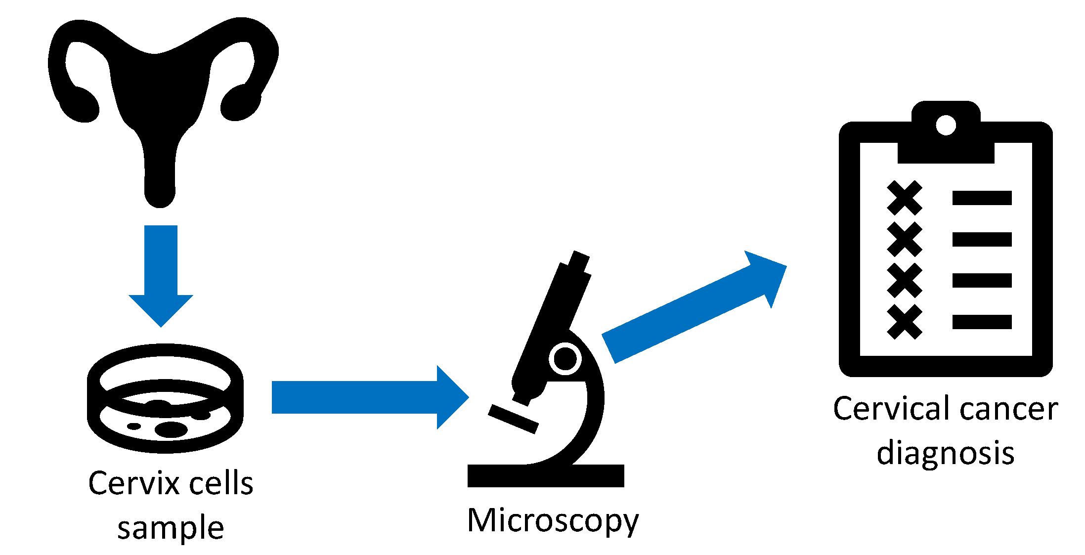
To confirm the diagnosis based on the results of the screening procedure, a colposcopy is performed. Colposcopy is a method of observing the surface of the cervix with a magnification of 6–40 times. It is an examination method for the vulva, vagina, and cervix. Colposcopy is performed with the help of a colposcope—a specially designed mobile microscope with a magnification of 2–40 times. Depending on whether the neck of the uterus (cervix) and vagina (Greek kolpos) are observed, the method is called colposcopy or vulvoscopy (if the external genitalia (vulva) is observed). A data flow of a colposcopic diagnostic procedure is presented in Figure 2.

Simple or native colposcopy means the simple observation of the cervix, and extended colposcopy implies the use of optical or chemical aids. The optical aid is a green filter that particularly improves the visualization of blood vessels on the surface of the cervix. Chemical aids used are $3\%$ acetic acid and Lugol’s solution (a solution of iodine in potassium iodate). Under the influence of acetic acid in areas of abnormal epithelium where there is a smaller number of intercellular bridges, and cellular connections/gap junctions, acetic acid penetrates cells more easily and causes the denaturation of cellular proteins. The result is the swelling of the cylindrical epithelium, which becomes anemic and gives the image of a white epithelium/acetobleaching, which is designated as a positive acetic reaction. By applying Lugol’s solution/Schiller’s test to the surface of the squamous epithelium, glycogen from the surface cells binds iodine from the solution, and the epithelium is stained dark brown—an iodine positive reaction. An iodine-positive reaction excludes the existence of epithelial cell atypia with great certainty. Different combinations of these reactions have different meanings in the assessment of changes on the cervical surface. The abnormal epithelium is usually white in color and does not receive iodine (iodine-negative changes). Colposcopy is an excellent diagnostic supplement to cytology. It enables a reliable assessment of the localization and extent of the pathological epithelial lesion, and a targeted biopsy from the suspicious area. The accuracy of colposcopy lies in the range of 60–85%, in combination with cytology 98–99%, and it is highly dependent on the colposcopist’s experience. The frequency of false-positive findings is estimated at $7\%$ and false-negative diagnoses at $13\%$ [36]. A biopsy is a procedure where the sampling of the suspicious parts of the cervix is performed with the following histological analysis [37].

2.2. AI-Based Tentative Screening for Cervical Cancer

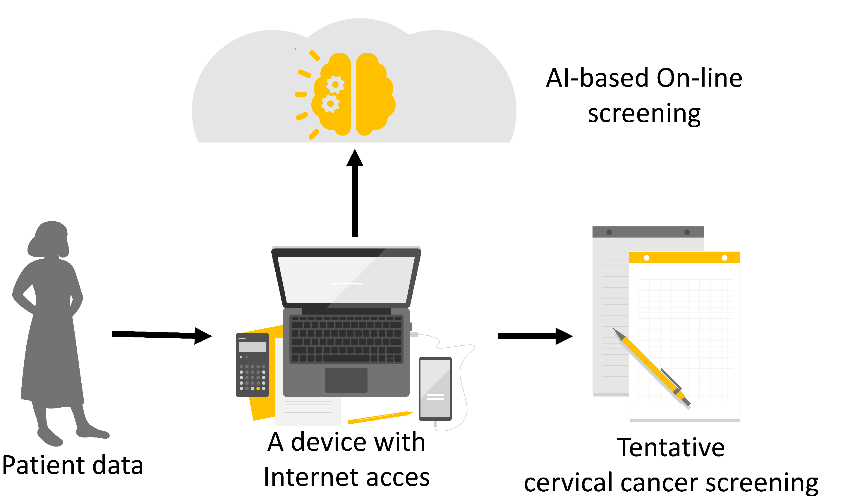
To increase cervical cancer screening rates and to enable questionnaire-based cervical cancer screening, the utilization of AI methods is proposed. The main idea is to use an AI algorithm to tentatively determine whether the patient has the possibility of suffering from cervical cancer, based on the survey questionnaire. In the described way, a significantly faster and more non-invasive initial diagnostic procedure is possible, which can serve as a preventive tool in the fight against cervical cancer by increasing screening rates and by possibly achieving a higher rate of cancer diagnosis in the primary stages. Furthermore, if the developed AI algorithms are used to construct an on-line survey, the tentative screening rates can be possible even higher. The graphical overview of the proposed method is presented in Figure 3.

3. Data Set Used

In this section, a brief description of the used data set is provided. Furthermore, the description of the proposed class-balancing techniques is given.

3.1. Data Set Description

The data set used in this research is the publicly available data set presented in [23]. The data set is collected at Hospital Universitario de Caracas in Venezuela, and at this time, it presents the only publicly available data set that can be used for the development of tentative cervical cancer screening based on questionnaire and AI algorithms. In this research, the data set will be used to determine the applicability of AI algorithms and class balancing techniques for the development of a survey for tentative cervical cancer screening.

The data set consists of 32 input variables and four output variables. The data set consists of 858 instances divided into 36 attributes. A detailed description of all input variables is presented in

Table 2. A brief description of input variables.

Variable	Type	Range
Age	int	13–84
Number of sexual partners	int	1–28
First sexual intercourse (age)	int	10–32
Number of pregnancies	int	0–11
Smoking	bool	0–1
Smoking	int	0–37
Smoking	int	0–37
Hormonal Contraceptives	bool	0–1
Hormonal Contraceptives (years)	int	0–22
IUD	bool	0–1
IUD	int	0–19
STDs	bool	0–1
STDs (number)	int	0–4
STDs: Condylomatosis	bool	0–1
STDs: Vaginal condylomatosis	bool	0–1
STDs: Vulvo-perineal condylomatosis	bool	0–1
STDs: Syphilis	bool	0–1
STDs: Pelvic inflammatory disease	bool	0–1
STDs: Genital herpes	bool	0–1
STDs: Molluscum contagiosum	bool	0–1
STDs: AIDS	bool	0–1
STDs: HIV	bool	0–1
STDs: Hepatitis B	bool	0–1
STDs: HPV	bool	0–1
STDs: Number of diagnosis	int	0–1
STDs: Time since first diagnosis	int	0–1
STDs: Time since last diagnosis	int	0–3
Dx: Cancer	bool	0–1
Dx: CIN	bool	0–1
Dx: HPV	bool	0–1
Dx	bool	0–1

.

The data set consists of four output variables, defined by using different diagnostic methods:

1

Biopsy [38],

2

Cytology [39],

3

Hinselmann [40],

4

Schiller [41].

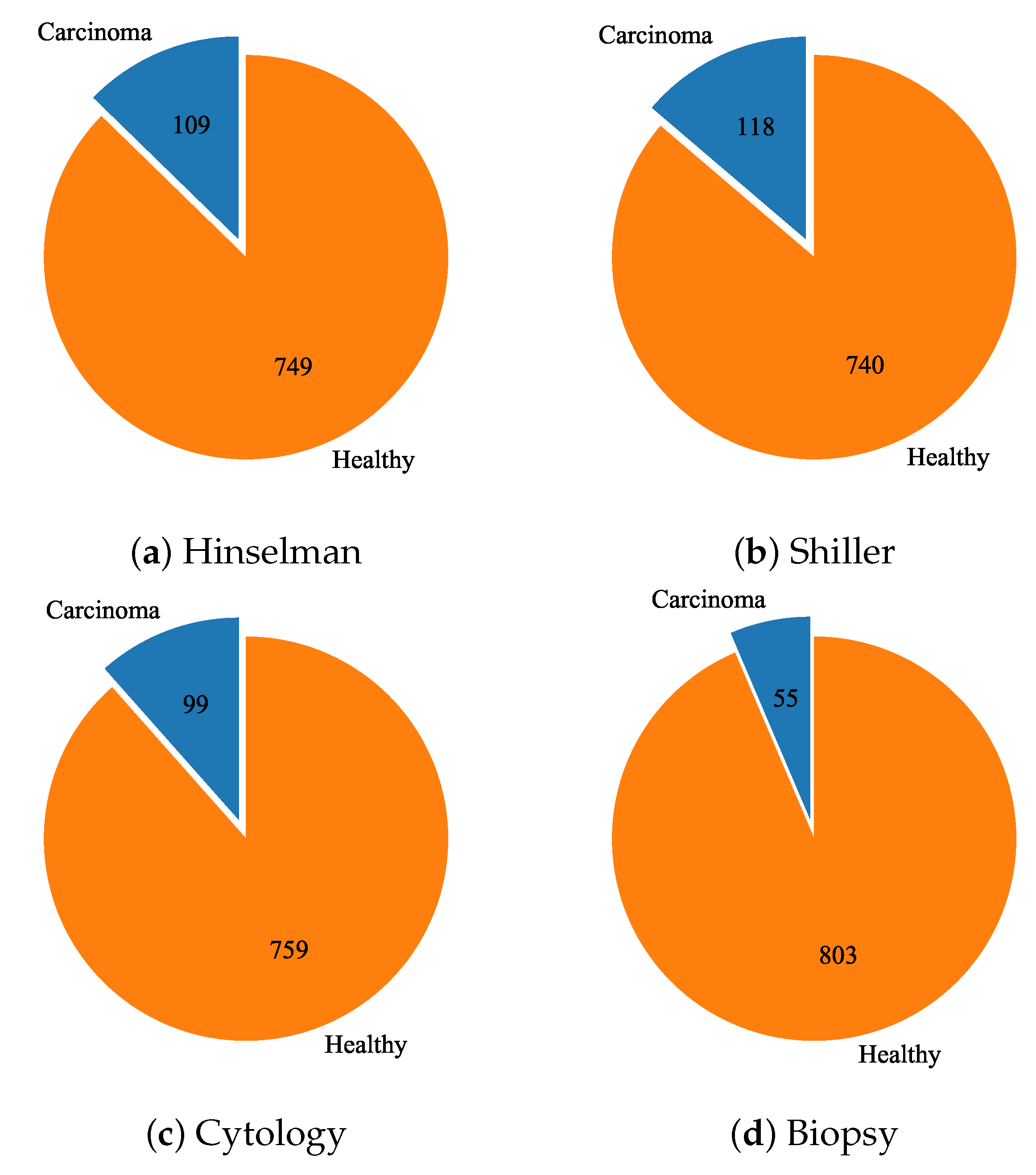
Each of the listed diagnostic methods represents a different output vector for the training of different classification algorithms. Each data set sample is paired with four bool values, one for each diagnostic method. The class distribution for each output vector is presented in Figure 4. From the presented distributions, it can be noticed that the data set is severely imbalanced. Due to the challenges of imbalanced data classification [42,43,44], several data set balancing techniques will be applied.

3.2. Class Balancing Techniques

As mentioned before, due to the significant class imbalanace in all four outputs, it is necessary to perform a certain form of class balancing techniques. In this research, class balancing techniques are applied to determine the best performing class balancing technique for this specific problem. In all cases, after the class balancing is performed, the resulting data set has a class distribution, with a ratio roughly equal to 50:50. In the following paragraphs, a brief description of class balancing techniques used in this research will be provided.

3.2.1. Random Oversampling

One of the basic methods for oversampling is random oversampling. With random oversampling, the samples in the minority class are randomly selected and duplicated, to match the number of samples in the majority class [45].

3.2.2. Synthetic Minority Oversampling Technique

Synthetic Minority Over-sampling Technique (SMOTE) is an oversampling method used to increase the number of samples that are contained in the minority class. The operational principle of SMOTE has its fundaments in the generation of synthetic data by using the K-nearest neighbors method. By using such an approach, it is possible to increase the number of members of the minority class by using the data generated in the feature space. In this research, SMOTE will be combined with Edited Nearest Neighbor (EEN) to form SMOTEEN [46], and Tomek, to form SMOTETOMEK [47].

3.2.3. ADAptive SYNthetic Algorithm

ADAptive SYNthetic algorithm (ADASYN) is an oversampling algorithm that can be described in several steps [48]. The first step is the calculation of the ratio between the number of minority and majority class members. Such a ratio can be defined as:

$$T=\frac{N_{min}}{N_{maj}}.$$

(1)

The fraction T is used for the initialization of the ADASYN algorithm. After the initialization, the number of required synthetic data is determined as:

$$G=(N_{maj}-N_{min})\beta ,$$

(2)

where $\beta$ represents the desired ratio after the data generation. In the neighborhood of each minority sample, a dominance of the majority sample ($r_i$) must be defined as:

$$r_i=\frac{N_{m}aj}{k},$$

(3)

where k represents the number of nearest neighbors. The next step is to determine the number of synthetic samples as:

$$G_i=G\cap r_i,$$

(4)

where $\cap r_i$ represents $r_i$ normalized by using:

$$\sigma \cap r_i=\frac{r_i}{\sigma i=1T_{min}}.$$

(5)

Each synthetic sample ($s_i$) of the minority is then determined by randomly choosing one of the K-nearest neighbors of each real minority sample, and by using the:

$$s_i=x_i+(x_{zi}-x_i)\lambda ,$$

(6)

where $(x_{zi}-x_i)$ represents the difference vector, and where $\lambda$ represents the randomly generated number between 0 and 1.

4. Machine Learning-Based Classification Algorithms

In this section, a brief overview of used ML-based classification algorithms will be provided.

4.1. Logistic Regression

Logistic regression represents a basic classification algorithm used in various classification problems. It uses the logistic function as a demarcation between two classes [49]. Such an approach can be utilized only for binary classification problems. The standard logistic function can be defined as:

$$p\left(x\right)=\frac{1}{1+e^{-\frac{x-\mu }{s}}},$$

(7)

where $\mu$ defines the center point of the logistic curve and s represents a scale parameter. The logistic function can also be written as:

$$p\left(x\right)=\frac{1}{e^{-({\beta }_0+{\beta }_{q}x)}},$$

(8)

where ${\beta }_0$ and ${\beta }_1$ represent the intercept and slope.

4.2. K-Nearest Neighbors

K-nearest neighbors (KNN) is a classification algorithm that can be used in multiple classifications and regression problems. For the case of the classification, a sample is classified into the majority class of its neighbors. For the case of this research, to optimize the performances of the proposed KNN algorithm, the number of nearest neighbors required for classification is varied. In this case, an algorithm that uses 1, 2, 5, 10, 20, 50, 100, 200, and 500 nearest neighbors, respectively, is used.

4.3. Multilayer Perceptron

Multilayer perceptron (MLP) consists of the input layer, multiple fully connected hidden layers, and an output layer. For this research, the grid-search procedure is performed to determine the MLP model with the highest classification performances [50]. The varied hyper-parameters are presented in

Table 3. List of all MLP hyper-parameters used during the grid-search procedure.

Hyper-Parameter	All Possible Values
Hidden layers	(10), (10, 10), (100,10), (100,100), (10, 10, 10), (100, 100, 10)
Solver	LBFGS, Adam, SGD
Activation function	Tanh, ReLU, Logistic

.

4.4. Support Vector Machine

Another method used for classification in this research is SVM. The SVM operation is based on the determination of the non-linear demarcation kernel that is defined by using the data contained in the training data set. For this research, multiple kernels are tested, alongside different coefficients and scaling values [51]. The detailed list of hyper-parameters used during the grid-search procedure is given in

Table 4. List of all SVM hyper-parameters used during the grid-search procedure.

Hyper-Parameter	All Possible Values
Kernel	Linear, Poly, RBF, Sigmoid
Coefficient	0.1, 1, 10, 100, 1000
Regularization	1, 0.1, 0.01, 0.001, 0.0001

.

4.5. Naive Bayes Classifier

Naive Bayes Classifier (NBC) is a probabilistic classifier based on the Bayes theorem. The main principle of all NBCs is that the features are classified independently from one another. To establish NBC, some elemental assumptions must be made:

• all features are independent,
• each feature is equally important to the final classification outcome.

All NBCs are based on the same principle with foundations in the Bayes theorem [52]. Bayes theorem can be defined with:

$$P\left(A\right|B)=\frac{P(A\cup B)}{P\left(B\right)},$$

(9)

that gives:

$$P\left(A\right|B)=\frac{P\left(A\right)·P\left(B\right|A)}{P\left(B\right)}.$$

(10)

In the case of both equations, P represents probability, A represent. In this research, multiple NBC approaches were used for the classification and diagnosis of cervical cancer, and these are:

• Gaussian Naive Bayes,
• Multinomial Naive Bayes,
• Complement Naive Bayes,
• Bernoulli Naive Bayes.

Gaussian NBC is based on the assumption that all classes contained in the data set have normal (Gaussian) distribution. Multinomial NBC is a special form of NBC that uses the multinomial distribution of each data feature. Complement NBC is based on the method that does not calculate the probability the belonging to a certain class, but rather, calculates the probability of belonging to each possible class. Bernoulli NBC is based on the assumption that all of the classes contained in the data set are distributed according to the Bernoulli distribution.

5. Research Methodology

To define the combination of an ML algorithm and class balancing technique that will produce the highest classification and generalization performances, the methodology based on a five-fold cross-validation is proposed. By using such an approach, the influence of specific data groups on the model performance will be neglected [53]. The schematic overview of the five-fold cross-validation process is presented in Figure 5.

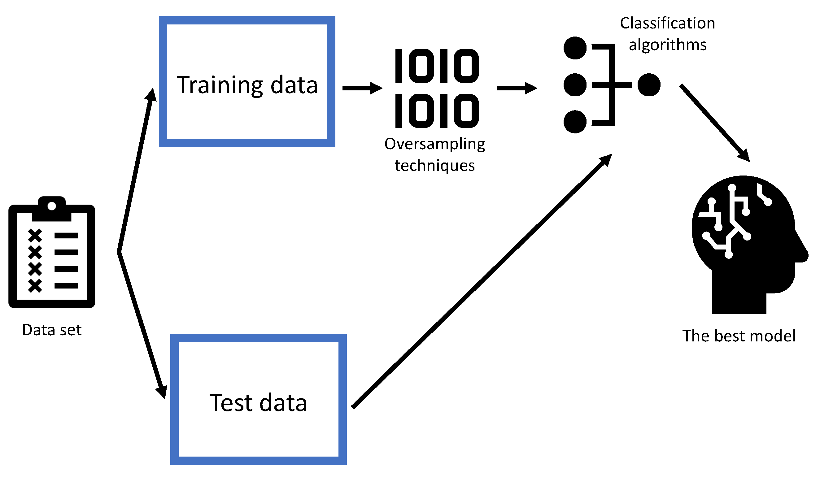
To determine the algorithm with optimal performances, for each case, in five-fold cross-validation, class balancing techniques will be applied to the training data set. On the other hand, the testing data set will remain the same. A graphical overview of the described process is given in Figure 6.

To quantify the classification performances, two different metrics are used. The first metric is widely used Area Under the ROC curve ($AUC$). $ROC$ curve is a curve constructed in the false positive rate ($FPR$)–true positive rate ($TPR$) plane, where $FPR$ is on the x, and $TPR$ on y axis. The $AUC$ is the area under the $ROC$ curve, and it represents a single, scalar value that can be used as a classification measure. $AUC$ represents a float value ranging from $0.5$ (random classification) to 1 (perfect classification) [50].

Another method that is used for the evaluation of classification performances is the Matthews Correlation Coefficient (MCC). MCC can be defined by using the data determined from the confusion matrix, as [54]:

$$MCC=\frac{TP·TN-FP·FN}{(TP+FP)(TP+FN)(TN+FP)(TN+FN)},$$

(11)

where $TP$ represent the number of truly positive sample, $FP$ represents the number of falsely positive samples, $TN$ represents the number of true negative samples and $TN$ represents the number of falsely negative samples. To define the performances from the results obtained from five-fold cross-validation, mean values, and standard deviation will be determined by using both described metrics.

6. Results and Discussion

In this section, results achieved with all four output variables will be presented. First, the results achieved with the original data set will be presented for each output variable. After the original data set, the results achieved with oversampled data sets will be presented and commented on. At the end of the section, the results will be compared and discussed.

6.1. Biopsy

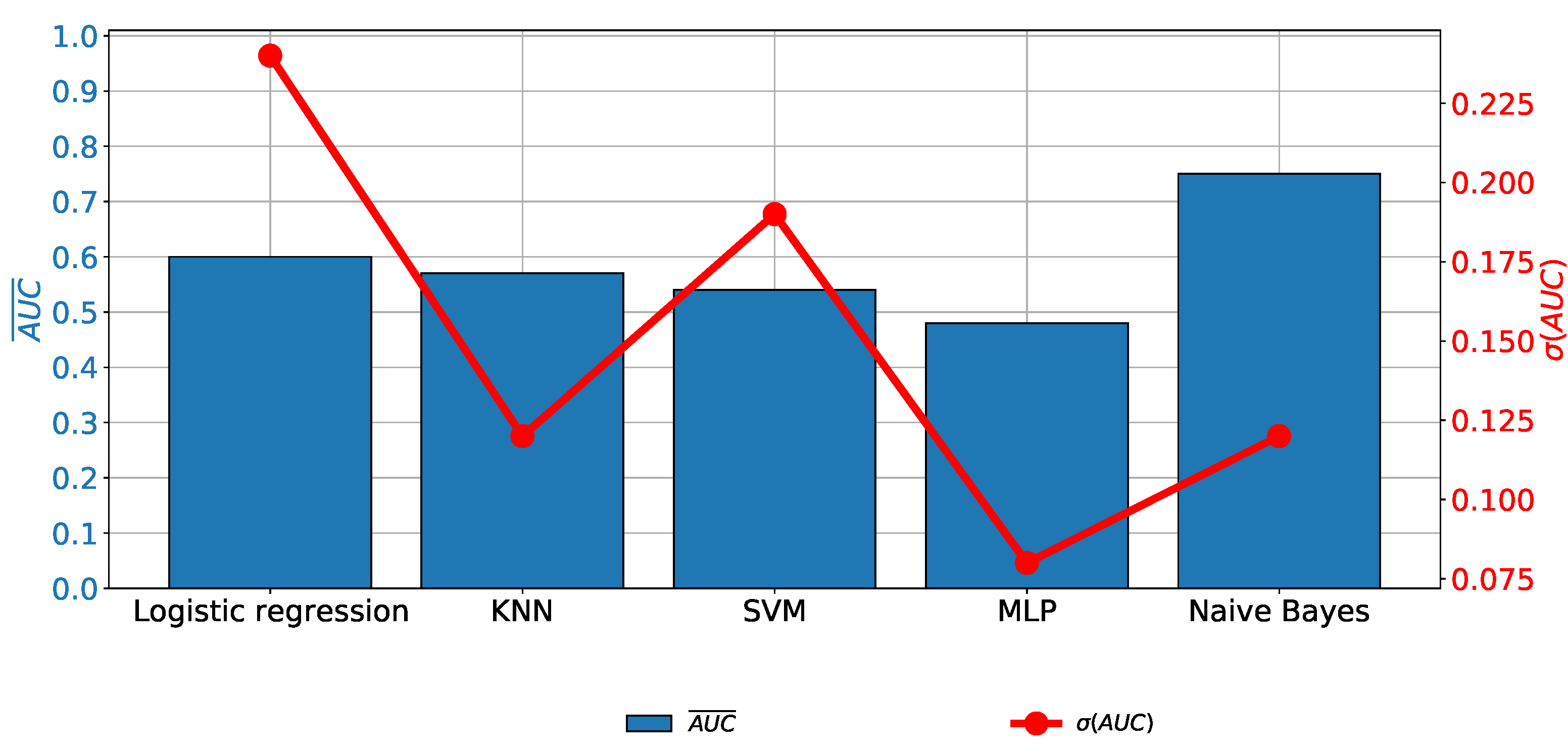
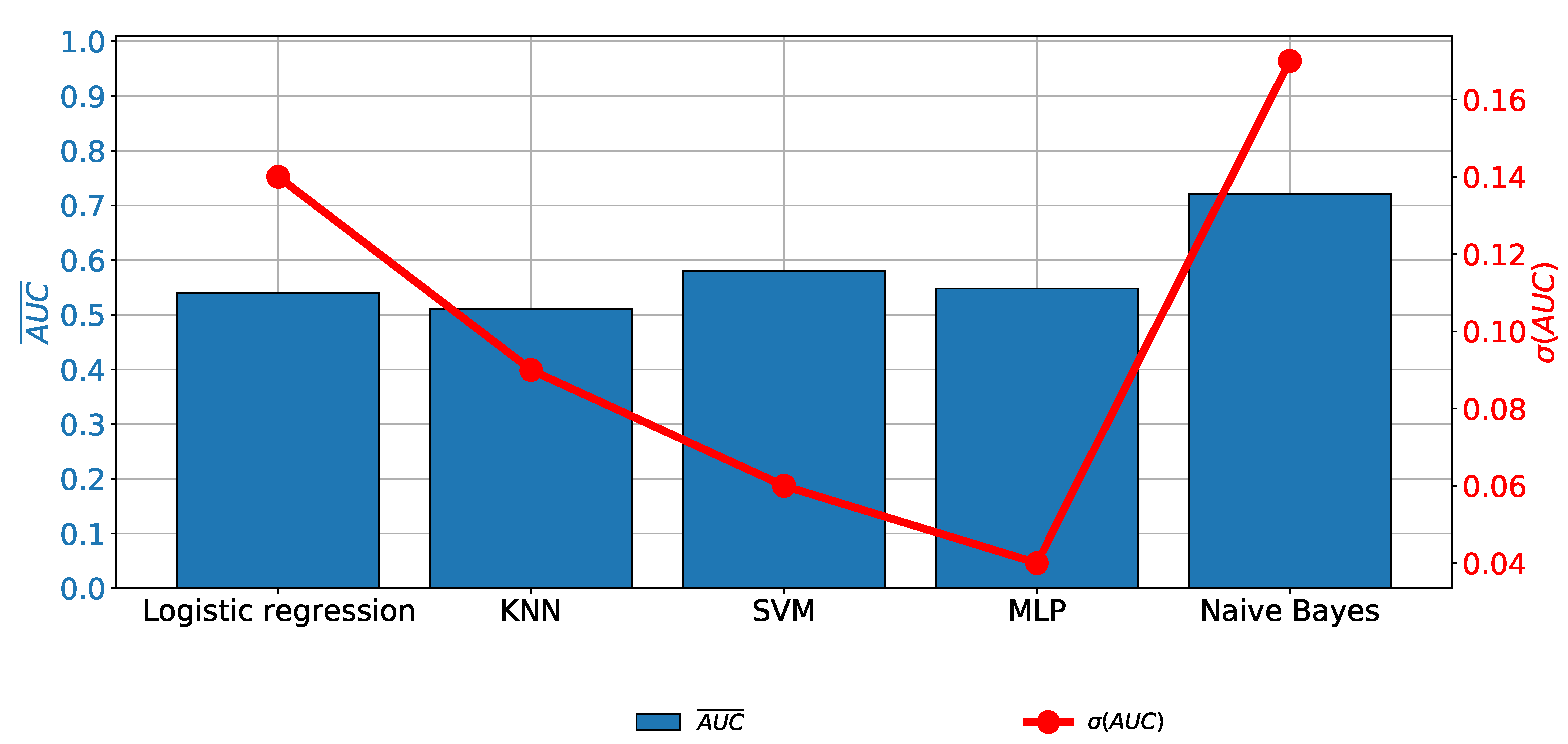
In the case of Biopsy data as the output variable, it can be noticed that no remarkable classification performances are achieved, regardless of the classifier used. A similar conclusion can be derived if generalization performances are observed. It can be noticed that an $\sigma \left(AUC\right)$ value of higher than $0.7$ is achieved only in the case of NBC, as presented in Figure 7.

When the class balancing techniques are applied, an increase in classification and generalization performances can be noticed. The highest classification and generalization performances are achieved if the KNN or MLP classifiers are used. Such a conclusion can be derived, regardless of the oversampling technique and evaluation metric, as presented in

Table 5. Results achieved with biopsy output.

Classifier	Class Balancing Technique	$\overline{\mathit{A}\mathit{U}\mathit{C}}$	$\mathit{\sigma }\left(\mathit{A}\mathit{U}\mathit{C}\right)$	$\overline{\mathit{M}\mathit{C}\mathit{C}}$	$\mathit{\sigma }\left(\mathit{M}\mathit{C}\mathit{C}\right)$
	Random oversampling	0.73	0.01	0.71	0.21
	SMOTE	0.63	0.02	0.26	0.01
Logistic regression	ADASYN	0.59	0.02	0.19	0.07
	SMOTEEN	0.63	0.06	0.26	0.08
	SMOTETOMEK	0.66	0.12	0.61	0.14
	Random oversampling	0.97	0.15	0.94	0.04
	SMOTE	0.87	0.13	0.73	0.26
KNN classifier	ADASYN	0.86	0.12	0.74	0.1
	SMOTEEN	0.98	0.06	0.96	0.05
	SMOTETOMEK	0.94	0.15	0.88	0.17
	Random oversampling	0.74	0.19	0.46	0.23
	SMOTE	0.68	0.18	0.39	0.20
SVM classifier	ADASYN	0.65	0.23	0.21	0.22
	SMOTEEN	0.71	0.26	0.66	0.24
	SMOTETOMEK	0.71	0.19	0.42	0.21
	Random oversampling	0.96	0.09	0.94	0.08
	SMOTE	0.89	0.12	0.88	0.09
MLP Classifier	ADASYN	0.91	0.07	0.89	0.07
	SMOTEEN	0.94	0.04	0.93	0.05
	SMOTETOMEK	0.93	0.08	0.91	0.07
	Random oversampling	0.72	0.02	0.69	0.03
	SMOTE	0.76	0.01	0.74	0.01
Naive Bayes classifier	ADASYN	0.79	0.01	0.77	0.01
	SMOTEEN	0.72	0.01	0.69	0.01
	SMOTETOMEK	0.64	0.01	0.61	0.01

.

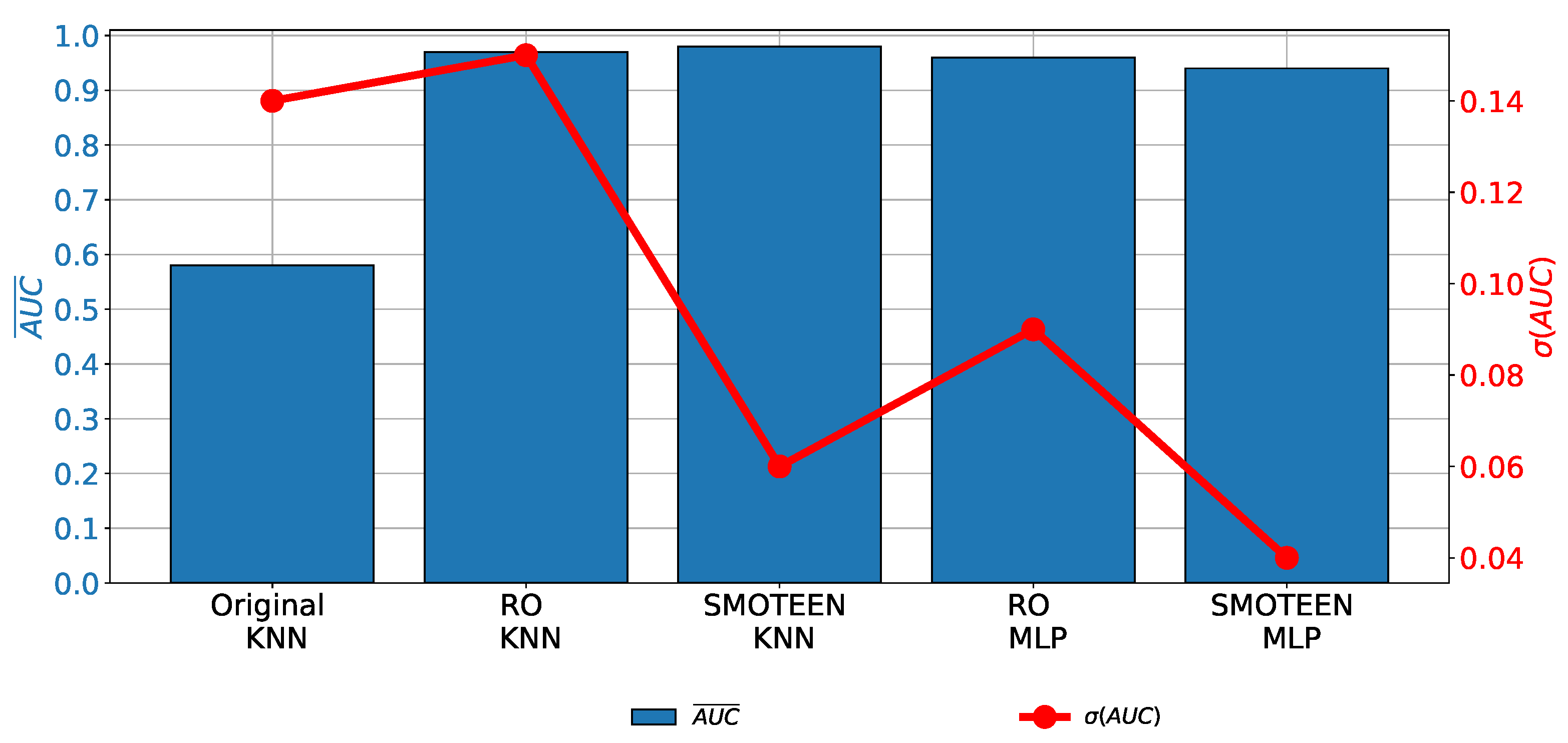
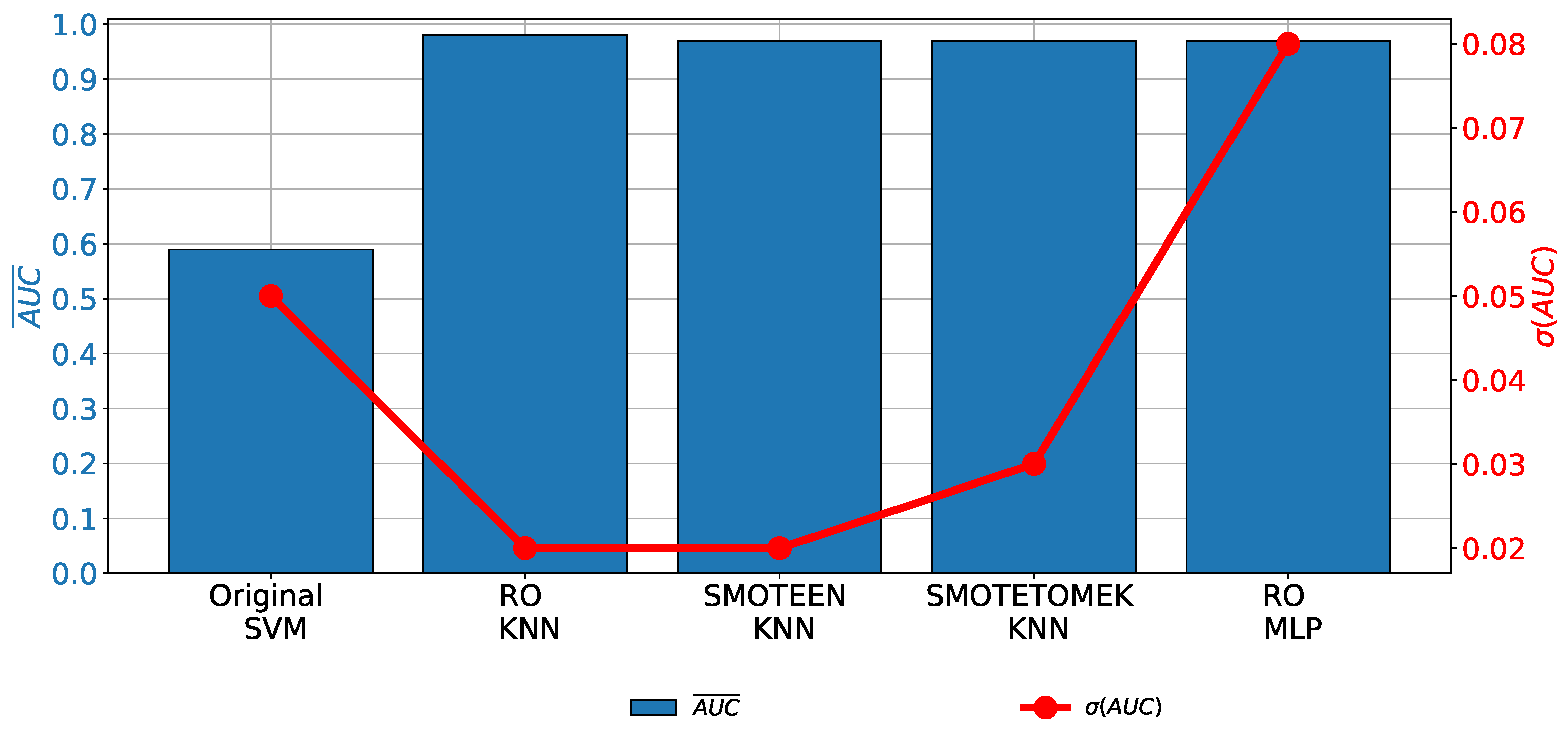
When the results achieved with the highest-performing combinations are compared with the results achieved with the original data set, it can be noticed that a significant increase in both classification and generalization performances is achieved (Figure 8).

The classifier hyper-parameters used in the highest-performing combinations are presented in

Table 6. List of hyper-parameters for highest-performing combinations in the case of Biopsy output.

Combination	Hyper-Parameters
RO-KNN	K = 250
SMOTEEN-KNN	K = 100
RO-MLP	(100, 100); LBFGS; ReLU
SMOTEEN-MLP	(100, 100); LBFGS; Logistic Sigmoid

.

6.2. Cytology

When the results achieved with the original data set that uses the Cytology variable as an output are observed, it can be noticed that none of the algorithms used has produced a classification performance of satisfying quality, as presented in Figure 9. For these reasons, it is concluded that is necessary to include class balancing techniques.

When class balancing techniques are applied, it can be seen that the classification performances that are higher than $0.9$ are achieved only if the MLP or KNN classifiers are used, as presented in

Table 7. Results achieved with cytology output.

Classifier	Class Balancing Technique	$\overline{\mathit{A}\mathit{U}\mathit{C}}$	$\mathit{\sigma }\left(\mathit{A}\mathit{U}\mathit{C}\right)$	$\overline{\mathit{M}\mathit{C}\mathit{C}}$	$\mathit{\sigma }\left(\mathit{M}\mathit{C}\mathit{C}\right)$
	Random oversampling	0.60	0.03	0.20	0.03
	SMOTE	0.73	0.02	0.46	0.02
Logistic regression	ADASYN	0.74	0.02	0.46	0.02
	SMOTEEN	0.75	0.03	0.49	0.03
	SMOTETOMEK	0.73	0.02	0.36	0.03
	Random oversampling	0.95	0.04	0.91	0.04
	SMOTE	0.89	0.09	0.77	0.08
KNN classifier	ADASYN	0.84	0.12	0.66	0.11
	SMOTEEN	0.92	0.05	0.84	0.05
	SMOTETOMEK	0.95	0.04	0.88	0.04
	Random oversampling	0.74	0.10	0.49	0.12
	SMOTE	0.69	0.14	0.64	0.13
SVM classifier	ADASYN	0.73	0.09	0.46	0.09
	SMOTEEN	0.73	0.19	0.38	0.24
	SMOTETOMEK	0.74	0.12	0.33	0.12
	Random oversampling	0.96	0.08	0.95	0.08
	SMOTE	0.87	0.04	0.87	0.04
MLP Classifier	ADASYN	0.88	0.07	0.88	0.04
	SMOTEEN	0.91	0.03	0.88	0.04
	SMOTETOMEK	0.92	0.03	0.89	0.03
	Random oversampling	0.71	0.21	0.52	0.19
	SMOTE	0.69	0.03	0.62	0.03
Naive Bayes classifier	ADASYN	0.70	0.03	0.70	0.03
	SMOTEEN	0.73	0.12	0.59	0.14
	SMOTETOMEK	0.77	0.10	0.69	0.12

. Such results are achieved only if Random oversampling, SMOTEEN, or SMOTETOMEK are used for class balancing.

By comparing the highest-performing combinations with the results achieved using the original data set, a significant increase in the classification and generalization properties are visible. The described comparison is presented in Figure 10.

The classifier hyper-parameters used in the highest-performing combinations are presented in

Table 8. List of hyper-parameters for highest-performing combinations in the case of cytology output.

Combination	Hyper-Parameters
RO-KNN	K = 100
SMOTEEN-KNN	K = 100
RO-MLP	(100, 100); LBFGS; Tanh
SMOTEEN-MLP	(100, 10); LBFGS; ReLU

.

6.3. Hinselmann

As it is in the case of biopsy and cytology, if the original data set with Hinselmann as the output variable is used, low classification and generalization performances are achieved. In this case, the $\sigma \left(AUC\right)$ value does not exceed 0.75, as presented in Figure 11.

When the class oversampling techniques are applied, it can be noticed that $\overline{AUC}$ and $\overline{MCC}$ values of higher than $0.9$ are achieved if KNN and MLP are used. In the case of KNN, three different combinations are achieving higher performances than MLP combined with random oversampling. The detailed results are presented in

Table 9. Results achieved with Hinselmann output.

Classifier	Class Balancing Technique	$\overline{\mathit{AUC}}$	$\mathit{\sigma }\left(\mathit{AUC}\right)$	$\overline{\mathit{MCC}}$	$\mathit{\sigma }\left(\mathit{MCC}\right)$
	Random oversampling	0.79	0.02	0.55	0.04
	SMOTE	0.78	0.05	0.49	0.06
Logistic regression	ADASYN	0.73	0.04	0.42	0.03
	SMOTEEN	0.79	0.03	0.50	0.06
	SMOTETOMEK	0.78	0.11	0.49	0.09
	Random oversampling	0.98	0.02	0.96	0.02
	SMOTE	0.97	0.04	0.92	0.05
KNN classifier	ADASYN	0.90	0.09	0.80	0.04
	SMOTEEN	0.97	0.02	0.94	0.02
	SMOTETOMEK	0.97	0.03	0.92	0.02
	Random oversampling	0.75	0.13	0.49	0.15
	SMOTE	0.86	0.19	0.64	0.21
SVM classifier	ADASYN	0.76	0.15	0.52	0.17
	SMOTEEN	0.80	0.13	0.47	0.12
	SMOTETOMEK	0.79	0.15	0.49	0.16
	Random oversampling	0.97	0.08	0.95	0.09
	SMOTE	0.94	0.07	0.93	0.06
MLP Classifier	ADASYN	0.94	0.02	0.94	0.02
	SMOTEEN	0.94	0.05	0.93	0.06
	SMOTETOMEK	0.94	0.03	0.92	0.04
	Random oversampling	0.61	0.02	0.58	0.02
	SMOTE	0.78	0.02	0.70	0.02
Naive Bayes classifier	ADASYN	0.76	0.01	0.68	0.01
	SMOTEEN	0.82	0.02	0.76	0.02
	SMOTETOMEK	0.80	0.01	0.72	0.02

.

If the results presented in Table 9 are compared with the results achieved on the original data set, it can be seen the $\sigma \left(AUC\right)$ values achieved with upsampled data sets are significantly higher, regardless of the classifier and class balancing techniques used. However, in the case of MLP trained with a randomly oversampled data set, $\sigma \left(AUC\right)$ is significantly higher, as presented in Figure 12. For these reasons, it can be concluded that KNN-based algorithms are characterized by higher generalization performances.

The hyper-parameters used to construct the above-presented classifiers are presented in

Table 10. List of hyper-parameters for highest-performing combinations in the case of Hinselmann output.

Combination	Hyper-Parameters
RO-KNN	K = 500
SMOTEEN-KNN	K = 250
SMOTETOMEK-KNN	K = 250
RO-MLP	(100, 100); LBFGS; Logistic Sigmoid

.

6.4. Shiller

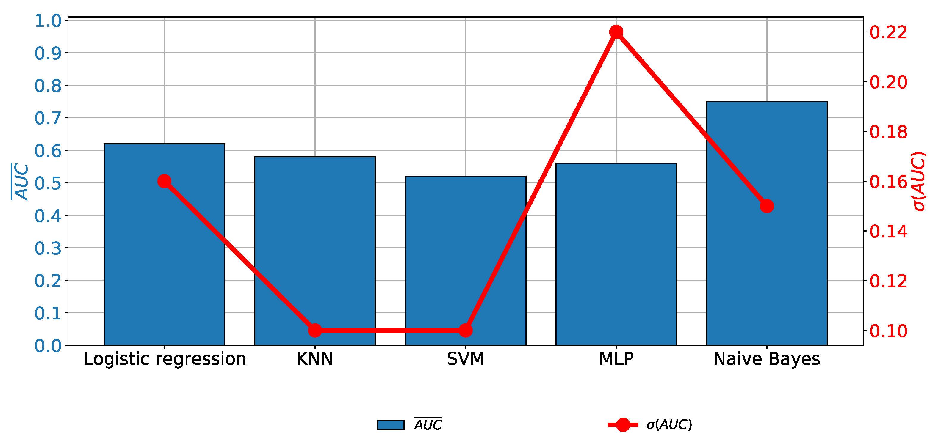
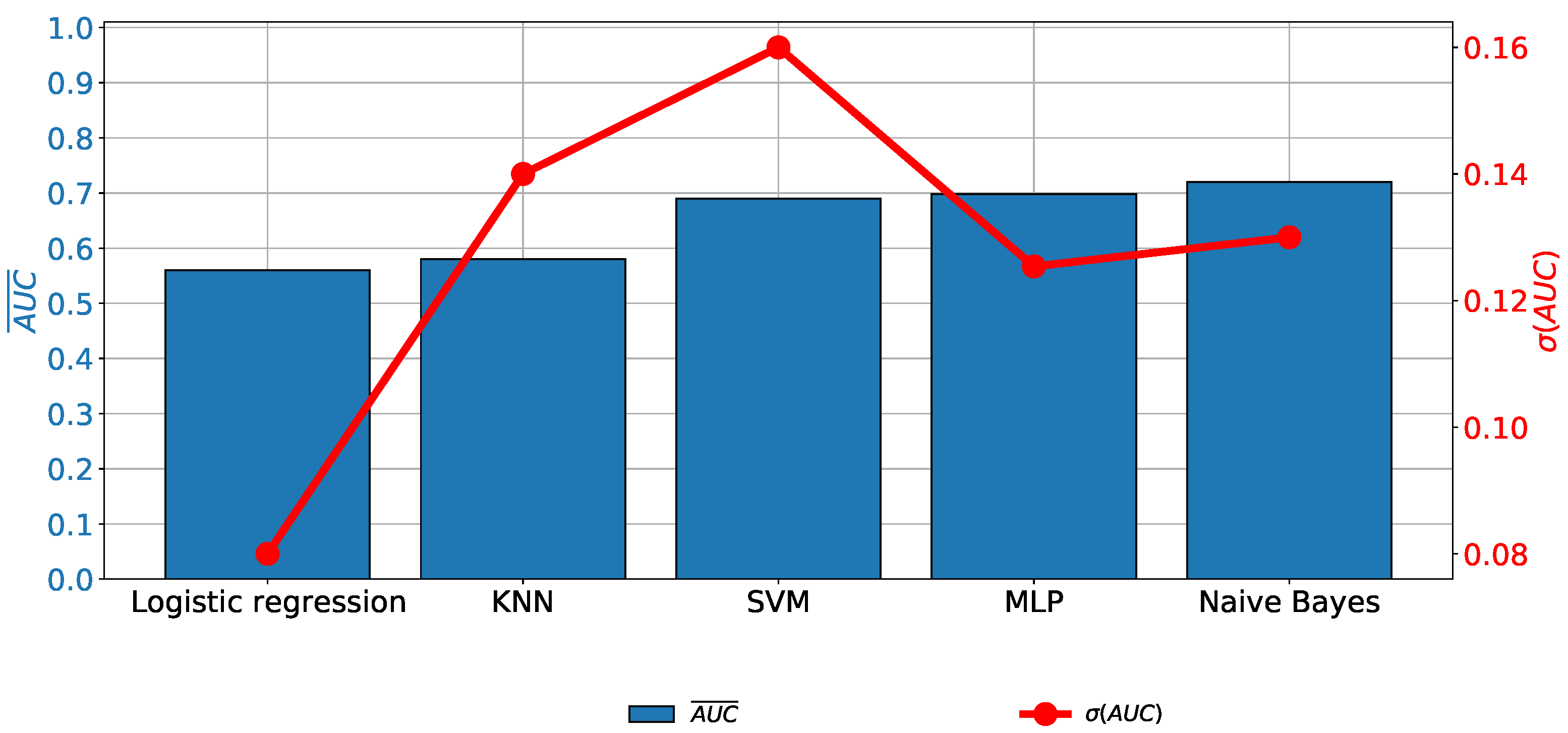
When the results achieved with the original data set that uses the Shiller variable as an output are compared, it can be seen that the $\sigma \left(AUC\right)$ does not exceed $0.75$, regardless of the algorithm used. It can be noticed that the highest results are achieved if SVM, MLP, or Naive Bayes are used, as presented in Figure 13.

When performances achieved with upsampled data sets are compared, it can be noticed that significantly higher $\overline{AUC}$ and $\overline{MCC}$ values are achieved if KNN and MLP models are trained by using random oversampling, SMOTEEN, and SMOTETOMEK. In the case of the listed combinations, $\overline{AUC}$ values of higher than $0.9$ are achieved. The detailed results are presented in

Table 11. Results achieved with Shiller output.

Classifier	Class Balancing Technique	$\overline{\mathit{AUC}}$	$\mathit{\sigma }\left(\mathit{AUC}\right)$	$\overline{\mathit{MCC}}$	$\mathit{\sigma }\left(\mathit{MCC}\right)$
	Random oversampling	0.63	0.14	0.33	0.12
	SMOTE	0.68	0.09	0.32	0.08
Logistic regression	ADASYN	0.61	0.07	0.21	0.08
	SMOTEEN	0.74	0.09	0.37	0.08
	SMOTETOMEK	0.60	0.14	0.15	0.07
	Random oversampling	0.94	0.06	0.89	0.05
	SMOTE	0.87	0.09	0.70	0.10
KNN classifier	ADASYN	0.84	0.07	0.69	0.07
	SMOTEEN	0.99	0.02	0.98	0.03
	SMOTETOMEK	0.98	0.02	0.92	0.02
	Random oversampling	0.69	0.17	0.38	0.17
	SMOTE	0.76	0.20	0.58	0.19
SVM classifier	ADASYN	0.62	0.08	0.24	0.08
	SMOTEEN	0.81	0.15	0.47	0.13
	SMOTETOMEK	0.79	0.13	0.38	0.14
	Random oversampling	0.92	0.06	0.91	0.06
	SMOTE	0.89	0.05	0.88	0.05
MLP Classifier	ADASYN	0.86	0.04	0.80	0.06
	SMOTEEN	0.94	0.04	0.92	0.04
	SMOTETOMEK	0.90	0.05	0.87	0.04
	Random oversampling	0.68	0.01	0.65	0.01
	SMOTE	0.75	0.02	0.72	0.02
Naive Bayes classifier	ADASYN	0.75	0.01	0.72	0.01
	SMOTEEN	0.71	0.01	0.62	0.01
	SMOTETOMEK	0.74	0.01	0.56	0.01

.

When the results achieved with the highest-performing combinations are compared with the results achieved with the original data set are compared, a significant increase in both classification and generalization performances can be noticed. However, a significant difference between the results achieved with KNN and MLP is noticeable. It can be seen that combinations designed with KNN have significantly higher classification and generalization performances, as presented in Figure 14.

The hyper-parameters used to construct the above-presented classifiers are presented in

Table 12. List of hyper-parameters for highest-performing combinations in the case of Shiller output.

Combination	Hyper-Parameters
RO-KNN	K = 100
SMOTEEN-KNN	K = 100
RO-MLP	(100, 100); LBFGS; Tanh
SMOTEEN-MLP	Logistic Sigmoid

.

6.5. Results Comparison and Discussion

According to the presented results, it can be seen that without the utilization of class-balancing techniques, low classification performances are achieved. In all cases, without the utilization of class-balancing techniques, classification close to coin-flip classification is achieved. Such low classification performances could be directly linked to the highly unbalanced data sets, with an extremely low number of positive samples. These low performances are the main reason for the impossibility of using AI algorithms to create a tentative screening for the diagnosis of cervical cancer. For these reasons, class-balancing techniques are considered and applied with aim of achieving higher classification performances.

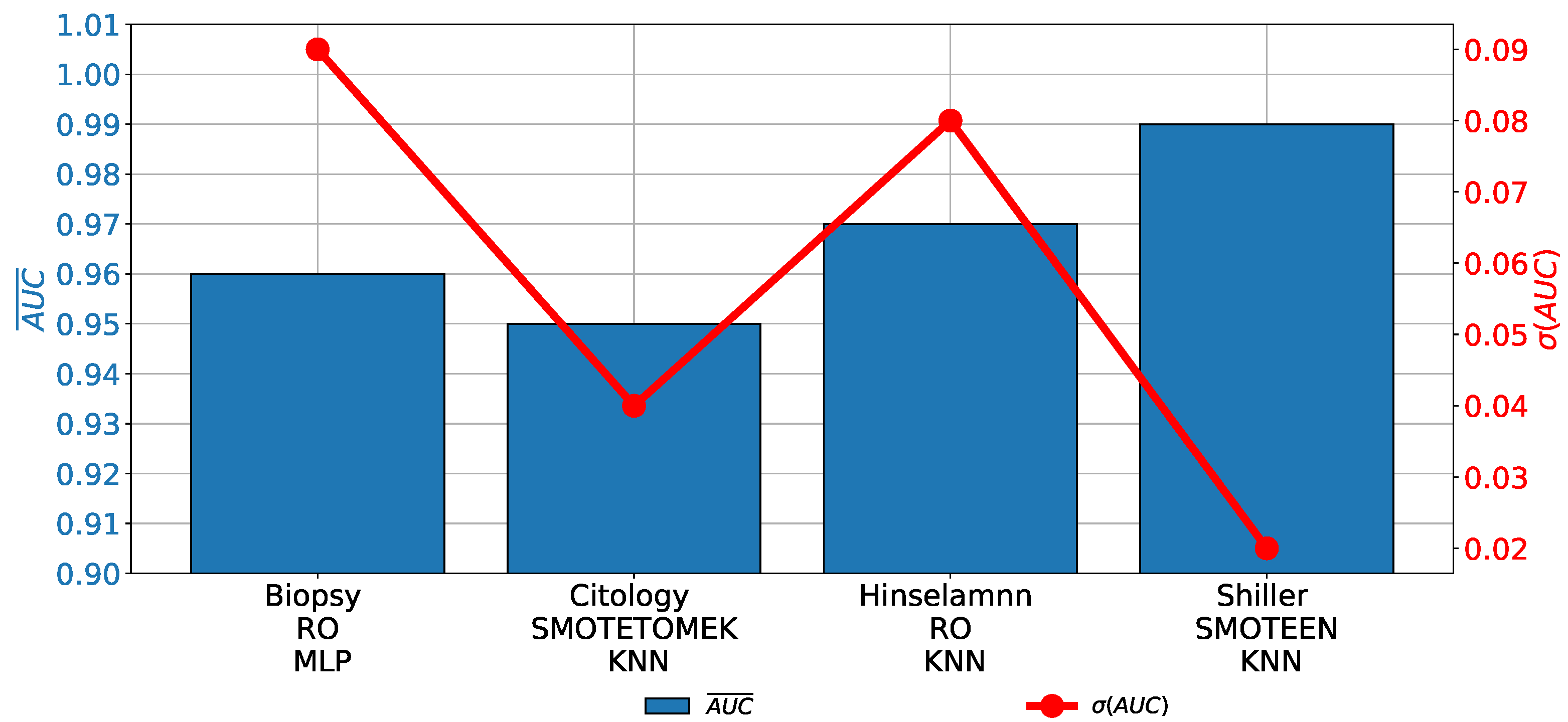
When the results achieved with the highest-performing combinations of AI classifiers and class-balancing methods are compared, it can be noticed that in all cases, $\overline{AUC}$ values over $0.95$ are achieved. Such results are showing high classification performances and they are pointing towards utilization possibility. Furthermore, in the case of Hinselmann and Shiller, even higher performances are achieved. Such a property can particularly be seen in the case of Shiller, where an $\overline{AUC}$ over $0.99$ is achieved, as presented in Figure 15. Furthermore, in this case, the lowest $sigma\left(AUC\right)$ values are achieved, pointing towards the highest generalization performances.

It can be noticed that in all cases, except when biopsy is used as the output variable, the highest classification and generalization performances are achieved if KNN is used. As can be seen from the results presented in Table 5, Table 7, Table 9 and Table 11, the high classification performances are achieved only if KNN or MLP are used as the main classification algorithm. In all other cases, the classification and generalization performances are significantly lower.

High classification performances achieved with multiple AI algorithms and multiple class-balancing techniques are pointing toward the conclusion that there is a possibility for the design of a redundant system that can use different methods to confirm the finding provided by the initial algorithm. Furthermore, this offers a possibility for the design of different classification ensembles that can further increase classification performances.

If the presented results are compared with the results presented in the state-of-the-art, it can be noticed that by using more advanced class balancing techniques such as SMOTEEN and SMOTETOMEK, a significant increase in both the classification and generalization performances can be noticed. Such a property is particularly emphasized in the cases of Hinselmann and Shiller. The main advantage of this research over the research presented in state-of-the-art is the examination of both-classification and generalization performances using the cross-validation method. Furthermore, the presented research is using appropriate classification quality metrics that can offer a single and scalar measure of classification quality and generalization performances.

7. Conclusions

In this article, class balancing techniques and ML methods are used to achieve cervical cancer diagnosis by using patient data. From the achieved results and by using the defined research hypothesis, the following conclusions can be derived:

• By using class balancing techniques, a significant increase in classification performances can be noticed.
• It can be noticed that by using random oversampling, SMOTEEN, and SMOTETOMEK, a significant increase in classification performances can be noticed.
• By using the SMOTETOMEK and SMOTEEN methods, a significant increase in generalization performances can be noticed.
• The presented results are pointing towards the conclusion that there is a possibility for the utilization of the developed methods for tentative cervical cancer screening.

The future work will be based on the development of an online survey that will be used as a tentative tool for cervical cancer screenings. To increase the performance of the proposed system, the new data set will be collected by using data from European clinics. During the collection of the new data, the possibility of the inclusion of new survey questions will also be investigated. From the AI standpoint, future work will include an investigation of the applicability of more complex class balancing techniques. Furthermore, future work will be based on the development of ensemble-based classifiers, whch will be used during the design of an online screening tool.

References

- Cohen, P.A.; Jhingran, A.; Oaknin, A.; Denny, L. Cervical cancer. Lancet 2019, 393, 169–182. [Google Scholar] [CrossRef]
- Buskwofie, A.; David-West, G.; Clare, C.A. A review of cervical cancer: Incidence and disparities. J. Natl. Med Assoc. 2020, 112, 229–232. [Google Scholar] [CrossRef]
- Vu, M.; Yu, J.; Awolude, O.A.; Chuang, L. Cervical cancer worldwide. Curr. Probl. Cancer 2018, 42, 457–465. [Google Scholar] [CrossRef]
- Waggoner, S.E. Cervical cancer. The lancet 2003, 361, 2217–2225. [Google Scholar] [CrossRef]
- Denny, L. Cervical cancer: Prevention and treatment. Discov. Med. 2012, 14, 125–131. [Google Scholar]
- Seoud, M.; Tjalma, W.A.; Ronsse, V. Cervical adenocarcinoma: Moving towards better prevention. Vaccine 2011, 29, 9148–9158. [Google Scholar] [CrossRef]
- Gien, L.T.; Beauchemin, M.C.; Thomas, G. Adenocarcinoma: A unique cervical cancer. Gynecol. Oncol. 2010, 116, 140–146. [Google Scholar] [CrossRef]
- Villa, L.L. Human papillomaviruses and cervical cancer. Adv. Cancer Res. 1997, 71, 321–341. [Google Scholar]
- Burd, E.M. Human papillomavirus and cervical cancer. Clin. Microbiol. Rev. 2003, 16, 1–17. [Google Scholar] [CrossRef] [Green Version]
- Issah, F.; Maree, J.E.; Mwinituo, P.P. Expressions of cervical cancer-related signs and symptoms. Eur. J. Oncol. Nurs. 2011, 15, 67–72. [Google Scholar] [CrossRef]
- Baser, E.; Togrul, C.; Ozgu, E.; Esercan, A.; Caglar, M.; Gungor, T. Effect of pre-procedural state-trait anxiety on pain perception and discomfort in women undergoing colposcopy for cervical cytological abnormalities. Asian Pac. J. Cancer Prev. 2013, 14, 4053–4056. [Google Scholar] [CrossRef] [Green Version]
- Wong, G.; Li, R.; Wong, T.; Fan, S. The effect of topical lignocaine gel in pain relief for colposcopic assessment and biopsy: Is it useful? BJOG: Int. J. Obstet. Gynaecol. 2008, 115, 1057–1060. [Google Scholar] [CrossRef]
- Michail, G.; Androutsopoulos, G.; Panas, P.; Valasoulis, G.; Papadimitriou, I.; Poulas, K.; Adonakis, G. Effects of Orally Administered Preliminary Analgesic Therapy in Diagnostic Colposcopy Patients: A Prospective Questionnaire Study. Open Med. J. 2021, 8, 1–7. [Google Scholar] [CrossRef]
- O’Laughlin, D.J.; Strelow, B.; Fellows, N.; Kelsey, E.; Peters, S.; Stevens, J.; Tweedy, J. Addressing anxiety and fear during the female pelvic examination. J. Prim. Care Community Health 2021, 12, 2150132721992195. [Google Scholar] [CrossRef]
- Zhang, S.; Xu, H.; Zhang, L.; Qiao, Y. Cervical cancer: Epidemiology, risk factors and screening. Chin. J. Cancer Res. 2020, 32, 720. [Google Scholar] [CrossRef]
- Bedell, S.L.; Goldstein, L.S.; Goldstein, A.R.; Goldstein, A.T. Cervical cancer screening: Past, present, and future. Sex. Med. Rev. 2020, 8, 28–37. [Google Scholar] [CrossRef]
- Guimarães, Y.M.; Godoy, L.R.; Longatto-Filho, A.; Reis, R.D. Management of early-stage cervical cancer: A literature review. Cancers 2022, 14, 575. [Google Scholar] [CrossRef]
- Maver, P.; Poljak, M. Primary HPV-based cervical cancer screening in Europe: Implementation status, challenges, and future plans. Clin. Microbiol. Infect. 2020, 26, 579–583. [Google Scholar] [CrossRef]
- MacLaughlin, K.L.; Jacobson, R.M.; Radecki Breitkopf, C.; Wilson, P.M.; Jacobson, D.J.; Fan, C.; St. Sauver, J.L.; Rutten, L.J.F. Trends over time in Pap and Pap-HPV cotesting for cervical cancer screening. J. Women’S Health 2019, 28, 244–249. [Google Scholar] [CrossRef]
- Watson, M.; Benard, V.; Flagg, E.W. Assessment of trends in cervical cancer screening rates using healthcare claims data: United States, 2003–2014. Prev. Med. Rep. 2018, 9, 124–130. [Google Scholar] [CrossRef]
- Sabatino, S.A.; White, M.C.; Thompson, T.D.; Klabunde, C.N. Cancer screening test use—United States, 2013. Morb. Mortal. Wkly. Rep. 2015, 64, 464. [Google Scholar]
- Lemp, J.M.; De Neve, J.W.; Bussmann, H.; Chen, S.; Manne-Goehler, J.; Theilmann, M.; Marcus, M.E.; Ebert, C.; Probst, C.; Tsabedze-Sibanyoni, L.; et al. Lifetime prevalence of cervical cancer screening in 55 low-and middle-income countries. JAMA 2020, 324, 1532–1542. [Google Scholar] [CrossRef] [PubMed]
- Fernandes, K.; Cardoso, J.S.; Fernandes, J. Transfer learning with partial observability applied to cervical cancer screening. In Proceedings of the Iberian Conference on Pattern Recognition and Image Analysis, Faro, Portugal, 20–23 June 2017; pp. 243–250. [Google Scholar]
- Geetha, R.; Sivasubramanian, S.; Kaliappan, M.; Vimal, S.; Annamalai, S. Cervical cancer identification with synthetic minority oversampling technique and PCA analysis using random forest classifier. J. Med. Syst. 2019, 43, 1–19. [Google Scholar] [CrossRef] [PubMed]
- Adem, K.; Kiliçarslan, S.; Cömert, O. Classification and diagnosis of cervical cancer with stacked autoencoder and softmax classification. Expert Syst. Appl. 2019, 115, 557–564. [Google Scholar] [CrossRef]
- Deng, X.; Luo, Y.; Wang, C. Analysis of risk factors for cervical cancer based on machine learning methods. In Proceedings of the 2018 5th IEEE International Conference on Cloud Computing and Intelligence Systems (CCIS), Nanjing, China, 23–25 November 2018; pp. 631–635. [Google Scholar]
- Ali, M.M.; Ahmed, K.; Bui, F.M.; Paul, B.K.; Ibrahim, S.M.; Quinn, J.M.; Moni, M.A. Machine learning-based statistical analysis for early stage detection of cervical cancer. Comput. Biol. Med. 2021, 139, 104985. [Google Scholar] [CrossRef]
- Abdoh, S.F.; Rizka, M.A.; Maghraby, F.A. Cervical cancer diagnosis using random forest classifier with SMOTE and feature reduction techniques. IEEE Access 2018, 6, 59475–59485. [Google Scholar] [CrossRef]
- Koss, L.G. The Papanicolaou test for cervical cancer detection: A triumph and a tragedy. JAMA 1989, 261, 737–743. [Google Scholar] [CrossRef]
- Denny, L. Cytological screening for cervical cancer prevention. Best Pract. Res. Clin. Obstet. Gynaecol. 2012, 26, 189–196. [Google Scholar] [CrossRef] [PubMed]
- De Villiers, E.M. Papillomavirus and HPV typing. Clin. Dermatol. 1997, 15, 199–206. [Google Scholar] [CrossRef]
- Gibb, R.K.; Martens, M.G. The impact of liquid-based cytology in decreasing the incidence of cervical cancer. Rev. Obstet. Gynecol. 2011, 4, S2. [Google Scholar]
- Denton, K.J. Liquid based cytology in cervical cancer screening. BMJ 2007, 335, 1–2. [Google Scholar] [CrossRef] [PubMed] [Green Version]
- Naucler, P.; Ryd, W.; Törnberg, S.; Strand, A.; Wadell, G.; Elfgren, K.; Rådberg, T.; Strander, B.; Johansson, B.; Forslund, O.; et al. Human papillomavirus and Papanicolaou tests to screen for cervical cancer. N. Engl. J. Med. 2007, 357, 1589–1597. [Google Scholar] [CrossRef] [PubMed]
- Mayrand, M.H.; Duarte-Franco, E.; Rodrigues, I.; Walter, S.D.; Hanley, J.; Ferenczy, A.; Ratnam, S.; Coutlée, F.; Franco, E.L. Human papillomavirus DNA versus Papanicolaou screening tests for cervical cancer. N. Engl. J. Med. 2007, 357, 1579–1588. [Google Scholar] [CrossRef] [PubMed] [Green Version]
- Dexeus, S.; Cararach, M.; Dexeus, D. The role of colposcopy in modern gynecology. Eur. J. Gynaecol. Oncol. 2002, 23, 269–277. [Google Scholar]
- Cafforio, P.; Palmirotta, R.; Lovero, D.; Cicinelli, E.; Cormio, G.; Silvestris, E.; Porta, C.; D’oronzo, S. Liquid biopsy in cervical cancer: Hopes and pitfalls. Cancers 2021, 13, 3968. [Google Scholar] [CrossRef]
- Ren, H.; Jia, M.; Zhao, S.; Li, H.; Fan, S. Factors correlated with the accuracy of colposcopy-directed biopsy: A systematic review and meta-analysis. J. Investig. Surg. 2022, 35, 284–292. [Google Scholar] [CrossRef]
- Fu, L.; Xia, W.; Shi, W.; Cao, G.; Ruan, Y.t.; Zhao, X.; Liu, M.; Niu, S.; Li, F.; Gao, X. Deep learning based cervical screening by the cross-modal integration of colposcopy, cytology, and HPV test. Int. J. Med. Inform. 2022, 159, 104675. [Google Scholar] [CrossRef]
- Nikookar, E.; Naderi, E.; Rahnavard, A. Cervical cancer prediction by merging features of different colposcopic images and using ensemble classifier. J. Med. Signals Sens. 2021, 11, 67. [Google Scholar]
- Afanasiev, M.S.; Dushkin, A.D.; Grishacheva, T.G.; Afanasiev, S.S. Photodynamic therapy for early-stage cervical cancer treatment. Photodiagnosis Photodyn. Ther. 2022, 37, 102620. [Google Scholar] [CrossRef]
- Patel, H.; Singh Rajput, D.; Thippa Reddy, G.; Iwendi, C.; Kashif Bashir, A.; Jo, O. A review on classification of imbalanced data for wireless sensor networks. Int. J. Distrib. Sens. Netw. 2020, 16, 1550147720916404. [Google Scholar] [CrossRef]
- Liu, H.; Zhou, M.; Liu, Q. An embedded feature selection method for imbalanced data classification. IEEE/CAA J. Autom. Sin. 2019, 6, 703–715. [Google Scholar] [CrossRef]
- Gupta, S.; Gupta, M.K. Computational prediction of cervical cancer diagnosis using ensemble-based classification algorithm. Comput. J. 2022, 65, 1527–1539. [Google Scholar] [CrossRef]
- Xin, L.K.; Rashid, N.b.A. Prediction of depression among women using random oversampling and random forest. In Proceedings of the 2021 International Conference of Women in Data Science at Taif University (WiDSTaif), Taif, Saudi Arabia, 30–31 March 2021; pp. 1–5. [Google Scholar]
- Kumar, V.; Lalotra, G.S.; Sasikala, P.; Rajput, D.S.; Kaluri, R.; Lakshmanna, K.; Shorfuzzaman, M.; Alsufyani, A.; Uddin, M. Addressing binary classification over class imbalanced clinical datasets using computationally intelligent techniques. Healthcare 2022, 10, 1293. [Google Scholar] [CrossRef] [PubMed]
- Wang, Z.; Wu, C.; Zheng, K.; Niu, X.; Wang, X. SMOTETomek-based resampling for personality recognition. IEEE Access 2019, 7, 129678–129689. [Google Scholar] [CrossRef]
- Anđelić, N.; Baressi Šegota, S.; Lorencin, I.; Glučina, M. Detection of Malicious Websites Using Symbolic Classifier. Future Internet 2022, 14, 358. [Google Scholar] [CrossRef]
- Schober, P.; Vetter, T.R. Logistic regression in medical research. Anesth. Analg. 2021, 132, 365. [Google Scholar] [CrossRef]
- Lorencin, I.; Anđelić, N.; Španjol, J.; Car, Z. Using multi-layer perceptron with Laplacian edge detector for bladder cancer diagnosis. Artif. Intell. Med. 2020, 102, 101746. [Google Scholar] [CrossRef] [PubMed]
- Mohammadi, M.; Rashid, T.A.; Karim, S.H.T.; Aldalwie, A.H.M.; Tho, Q.T.; Bidaki, M.; Rahmani, A.M.; Hosseinzadeh, M. A comprehensive survey and taxonomy of the SVM-based intrusion detection systems. J. Netw. Comput. Appl. 2021, 178, 102983. [Google Scholar] [CrossRef]
- Phoenix, P.; Sudaryono, R.; Suhartono, D. Classifying promotion images using optical character recognition and Naïve Bayes classifier. Procedia Comput. Sci. 2021, 179, 498–506. [Google Scholar]
- Lorencin, I.; Anđelić, N.; Mrzljak, V.; Car, Z. Genetic algorithm approach to design of multi-layer perceptron for combined cycle power plant electrical power output estimation. Energies 2019, 12, 4352. [Google Scholar] [CrossRef] [Green Version]
- Chicco, D.; Jurman, G. The advantages of the Matthews correlation coefficient (MCC) over F1 score and accuracy in binary classification evaluation. BMC Genom. 2020, 21, 6. [Google Scholar] [CrossRef] [PubMed]
Figure 1.
The comparison of maximal and rates achieved with PAP, LBC, and HPV-DNA testing.
Figure 2.
An illustration of the colposcopy procedure.
Figure 3.
A schematic representation of the proposed method for tentative cervical cancer screening.
Figure 4.
The class distribution for each output variable (a) Hinselman; (b) Shiller; (c) Cytology, (d) Biopsy.
Figure 5.
The schematic overview of the 5-fold cross-validation process.
Figure 6.
The research methodology for one case in 5-fold cross validation.
Figure 7.
The results achieved with the original data set and biopsy output.
Figure 8.
Comparison of the highest results achieved with original and balanced data set for the case of Biopsy output.
Figure 9.
The results achieved with the original data set and cytology output.
Figure 10.
Comparison of the highest results achieved with original and balanced data set for the case of cytology output.
Figure 11.
The results achieved with original data set and Hinselmann output.
Figure 12.
Comparison of the highest results achieved with original and balanced data set for the case of Hinselmann output.
Figure 13.
The results achieved with original data set and Shiller output.
Figure 14.
Comparison of the highest results achieved with original and balanced data set for the case of Shiller output.
Figure 15.
Comparison of the achieved results.