
Combining a Universal OBD-II Module with Deep Learning to Develop an Eco-Driving Analysis System


1
Department of Electronic Engineering, National Chin-Yi University of Technology, Taichung 41170, Taiwan
2
CANDOMO Technology Corporation Limited, Taichung 423, Taiwan
*
Author to whom correspondence should be addressed.
Appl. Sci. 2021, 11(10), 4481; https://doi.org/10.3390/app11104481
Submission received: 20 April 2021
/
Revised: 11 May 2021
/
Accepted: 12 May 2021
/
Published: 14 May 2021
(This article belongs to the Section Computing and Artificial Intelligence)
Abstract
:Vehicle technology development drives economic development but also causes severe mobile pollution sources. Eco-driving is an effective driving strategy for solving air pollution and achieving driving safety. The on-board diagnostics II (OBD-II) module is a common monitoring tool used to acquire sensing data from in-vehicle electronic control units. However, different vehicle models use different controller area network (CAN) standards, resulting in communication difficulties; however, relevant literature has not discussed compatibility problems. The present study researched and developed the universal OBD-II module, adopted deep learning methods to evaluate fuel consumption, and proposed an intuitive driving graphic user interface design. In addition to using the universal module to obtain data on different CAN standards, this study used deep learning methods to analyze the fuel consumption of three vehicles of different brands on various road conditions. The accuracy was over 96%, thus validating the practicability of the developed system. This system will greatly benefit future applications that employ OBD-II to collect various types of driving data from different car models. For example, it can be implemented for achieving eco-driving in bus driver training. The developed system outperforms those proposed by previous research regarding its completeness and universality.
1. Introduction
Eco-driving ameliorates unsafe driving behaviors and styles, achieving safe driving with reduced energy consumption [1]. Factors affecting fuel consumption and driving safety include calm driving styles, maintenance of a safe driving speed, proper use of air conditioning, and optimal route planning. Therefore, the definition of factors affecting fuel consumption is fundamental to achieving eco-driving. Excessive acceleration, deceleration, and high-speed driving should be avoided to reduce fuel consumption [2], as should the use of low gears and frequent gear shifting [3]. The literature has classified driving styles into ordinary, calm, aggressive, or unnatural according to various driving parameters, including vehicle speed, acceleration, engine speed, and driving duration [4]. Aggressive or unnatural driving styles lead to higher fuel consumption, exacerbate environmental pollution, and directly influence driving safety [5]. Accordingly, multiple studies have proposed methods to achieve safe [6,7], economical [8,9], and comfortable [10] eco-driving.
Studies have revealed that the practice of monitoring and evaluating driving data to improve driving behavior has received increasing popularity and produced favorable results. The current monitoring tools predominantly employ standardized on-board diagnostics II (OBD-II) modules to obtain sensing data from the internal electronic control units (ECUs); the data are then converted into driving suggestions on the practice of eco-driving. OBD-II modules facilitate the acquisition of more accurate driving data than external sensors do; furthermore, they have a standardized connection interface and are convenient to install. Since 2008, all vehicles equipped with OBD-II communication interfaces have employed a controller area network (CAN bus) as the main architecture for the internal communication network [11,12]. The CAN bus is mainly used as the communication protocol in heavy-duty commercial vehicles and sedans, which respectively use CAN2.0A (an 11-bit identifier) and CAN2.0B (a 29-bit identifier). Vehicles of different types may have a baud rate of either 500 or 250 Kbp, along with a communication protocol of either ISO-15031 [13], ISO-27145 [14], or SAE-J1939 [15]. Devices with different CAN standards cannot communicate. To date, studies have not discussed the compatibility between CAN busses. Therefore, a universal OBD-II module will greatly increase the practice of eco-driving. The present study proposes an eco-driving assistant system to improve driving behaviors and encourage eco-driving. This system contains a universal OBD-II module capable of obtaining information from different CAN standards and employs deep learning to predict fuel consumption, thereby increasing the applicability and adoption of the eco-driving assistant system. The contributions of the study are:
- A universal OBD-II module is developed to collect driving information from various car models.
- Three deep learning methods are combined with the universal OBD-II module to predict fuel consumption.
- Three different car models are used to evaluate fuel consumption.
- An intuitive driving graphic user interface is designed for the eco-driving assistant system.
The rest of the paper is organized as follows. The related research is discussed in Section 2. The proposed eco-driving assistant system is described in Section 3, including the universal OBD-II module, graphical user interface, deep learning algorithms, and the test of three cars. The results and a related discussion are presented in Section 4 and Section 5, respectively. The conclusions are presented in Section 6.
2. Related Research
The development of vehicle technology drives economic development in various countries but also creates severe mobile pollution sources [16]. For example, CO2 emissions cause the greenhouse effect; SO2 and NOx cause acid rain and pulmonary diseases [17]. The European Union has established regulations to reduce greenhouse gas emissions by 32% by 2030 [18]. Vehicle CO2 emissions, which originate from the burning of fossil fuels, are directly related to fuel consumption [19]. Accordingly, CO2 reduction is considered a global goal. Eco-driving, a novel vehicle driving technology, adopts intelligent and safe driving to cut fuel consumption and reduce greenhouse gas emissions, traffic accidents, and noise [20]. Studies have indicated that eco-driving reduces fuel consumption and emissions by 10–25% [21,22,23,24,25] and also reduces greenhouse gas emissions by 30% [26].
Contemporary methods for promoting eco-driving consist of two types. First, holding education courses to improve driving behavior and methods [11]. In [12], an eco-driving course was held for drivers and modified according to drivers’ feedback; fuel consumption was reduced by 4.8%. Second, employing driving assistance systems to promptly indicate or correct unsafe driving behavior. These systems are further divided into factory-installed products and aftermarket-installed products. Factory-installed systems, in which the engine parameters are monitored remotely, include General Motors’ Onstar, BMW’s Connected Drive, and Lexus’s Link. In terms of the aftermarket-installed products, an OBD-II module is employed to acquire, analyze, and make suggestions based on the ECU parameters to reduce fuel consumption [27,28,29,30]. Meseguer et al. collected and evaluated vehicle speed, acceleration, engine speed, mass flow sensor (MAF), manifold absolute pressure (MAP), and intake air temperature (AIT) with an OBD-II module to determine driving styles and route types; with a focus on the relationship between driving behavior and fuel consumption, they reduced fuel consumption and greenhouse gas emissions [26]. Magana et al. employed fuzzy logic to integrate OBD-II, a GPS, and climate data to provide driving advice and achieved fuel savings of 11.04% [25]. Therefore, this type of smart assistance (neural network) system integration is a crucial direction in eco-driving research.
Studies have discussed implementing neural network assistance in eco-driving systems. Multiple frameworks of neural networks are available for selection based on the required data type and system demands. Ahn developed a regression model based on vehicle speed and acceleration; through using different regression coefficients under various driving conditions, the optimal model sum of squared errors (SSE) was achieved [31]. Ping et al. used object detection to convert the external environment into processable data, which were then used as the input for a clustering model. Through connecting dynamic environmental data with data on vehicle operation signals for analysis, their model achieved a prediction accuracy of over 80% [32]. Yao et al. used a back propagation neural network on smartphones and OBD-II devices to acquire data on driver behavior and fuel consumption and then explored their correlation [30]. Singh et al. adopted Elman neural network-based energy management strategies (EMSs) to determine the fuel efficiency of optimized hybrid electric vehicles [33]. The aforementioned research indicates that neural networks have achieved outstanding performance as eco-driving analysis tools. Therefore, the present study referred to fuel consumption prediction models proposed by previous research and adjusted the parameters to obtain a model framework that could accurately predict fuel consumption.
3. Materials and Methods
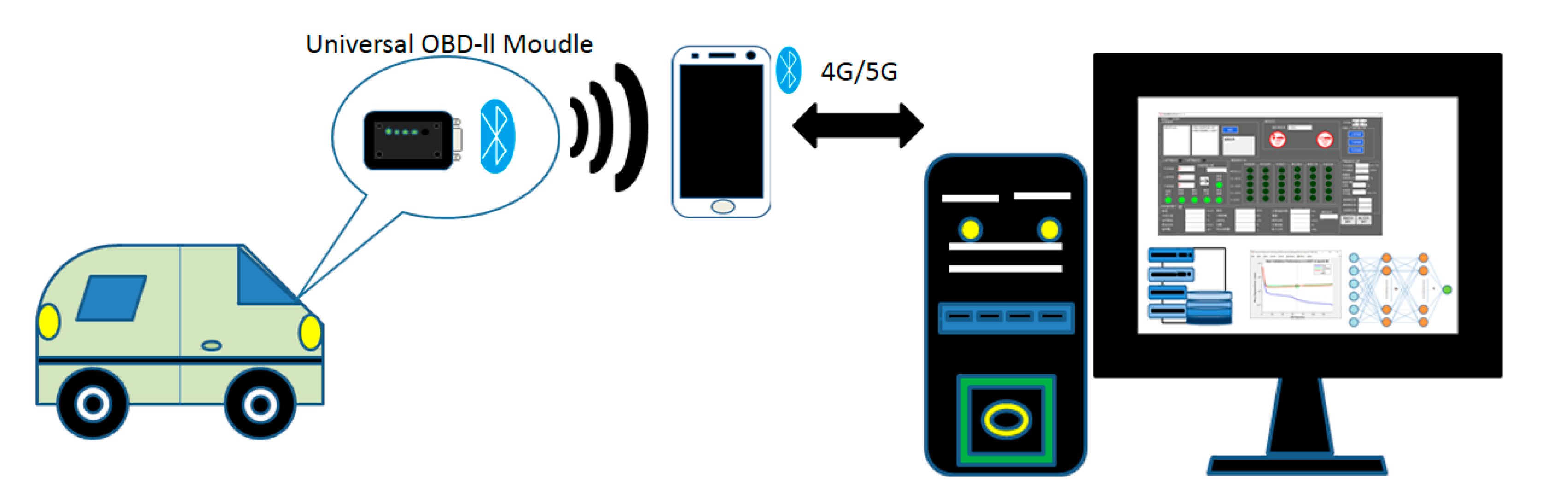
The developed system is presented in Figure 1. The proposed universal OBD-II module reads the in-vehicle driving data and transmits them through Bluetooth to a smartphone, which then transmits the data to a computer database, which is then used for subsequent analysis through deep learning.
3.1. Development of Universal OBD-II Hardware
To develop a universal product for different car brands and models, in addition to integrating the software communication protocols, the hardware functions must be developed accordingly to meet user needs. Figure 2 displays the universal OBD-II hardware, which consists of the K-line and CAN bus interface circuits for communicating with in-vehicle ECUs. A microprocessor (Model: PIC18F46K80) is used to acquire driving data, which are subsequently sent to the smartphone and computer ends using a Bluetooth module. K-line, a common diagnostic interface in early European and Japanese car models, is employed to ensure compatibility with older car models. The present study focused on the communication integration of the CAN bus.
3.2. Heterogenous Communication Protocol Identification in the CAN Bus
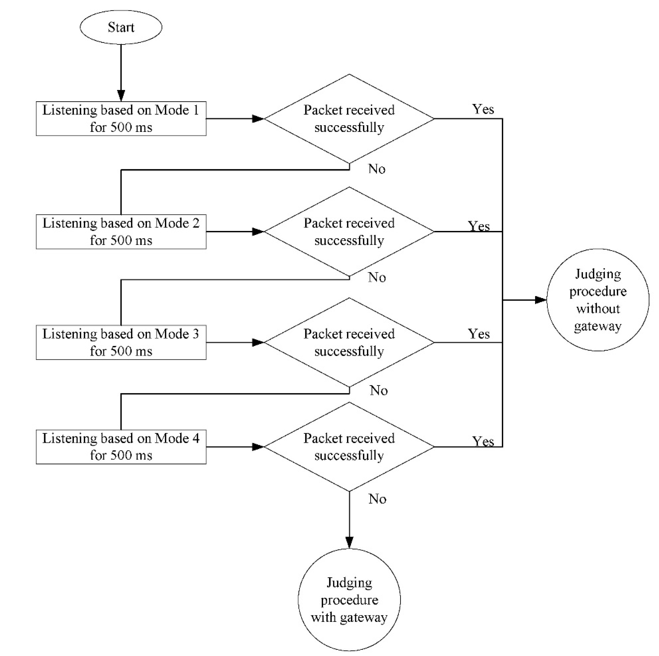
The integration of CAN bus communication protocols—namely, SAE-J1939, ISO-15031, and ISO-27145—involves identifying the communication protocol used in the car model in question. However, when using the communication characteristics of the CAN bus to determine the communication protocol, incorrect packets may result in the CAN bus entering the OFF state, which would halt the vehicle’s communication and result in the system crashing. Therefore, a listening mode is first used to examine the packet format for communication and to determine the protocol used. Figure 3 presents the initial determination procedures in listening mode, which is used to determine whether the received CAN bus packet is the correct one. In Modes 1, 2, 3, and 4, the determination criteria are set as CAN packets with a 29-bit ID and 500 kbps, an 11-bit ID and 500 kbps, a 29-bit ID and 250 kbps, and an 11-bit ID and 250 kbps, respectively. If a CAN bus packet is received, the procedure displayed in Figure 4 commences—namely, the diagnostic mode for vehicle communication modes without gateways. For vehicles whose communication diagnosis has gateways, the procedure in Figure 5 is involved instead. The communication diagnosis procedure in Figure 4 employs a service request packet to determine whether a vehicle has a particular communication protocol. In the procedure, a 29-bit communication mode is first adopted for the diagnosis of the SAE-J1939 protocol, followed by the diagnosis of the ISO-27145 and ISO-15031 protocols.
Figure 4 presents the communication diagnosis mode without gateways. The mode begins with determining whether the identifier code of the received packet is 29 bits. If so, the communication node is determined to have the SAE-J1939 protocol. The controller subsequently sends a request packet with a 29-bit identifier code to confirm whether the communication node contains another communication protocol. If the node contains the 29-bit ISO-27145 or ISO-15031 protocol, a feedback packet will be received. If a 29-bit feedback packet is not received after a request packet corresponding to the ISO-27145 or ISO-15031 protocol is sent, the system will then transmit an 11-bit request packet corresponding to the ISO-27145 and ISO-15031 protocols. This is because Japanese car models use 11-bit CAN busses as communication packets in their ECUs, whereas a 29-bit communication mode is used in the diagnosis. The aforementioned procedure facilitates the determination of whether a vehicle has two communication protocols. If the model receives a packet that is not 29 bits, then the communication node does not contain the SAE-J1939 protocol. Therefore, by transmitting an 11-bit request packet with the controller, the procedure can be used to determine whether the communication node contains the 11-bit ISO-27145 or ISO-15031 protocol.
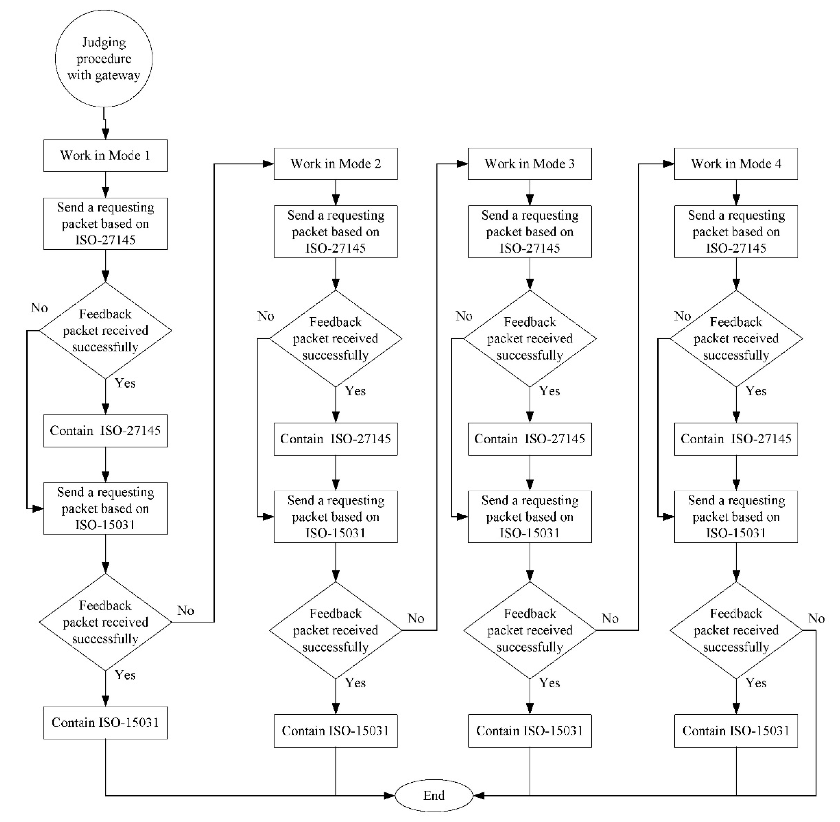
Figure 5 displays the procedure implemented if no packets are successfully received in either mode presented in Figure 3. In Figure 5, the CAN first works in Mode 1 and uses that mode’s settings to send a request packet based on the ISO-27145 protocol. The parameter ID (PID) of the communication node is then requested, and the communication is activated. If a feedback packet from the node is received, then the communication node is determined to contain the ISO-27145 protocol. Regardless of whether a feedback packet is received, a request packet based on ISO-15031 will be sent to request the PID of the communication node and to activate communication. If a feedback packet is received from the node, then the node is determined to contain the ISO-15031 protocol. If no feedback packets are received, the CAN performs Mode 2 and continues to confirm the communication protocol of the communication node by following the aforementioned procedure to complete Modes 1, 2, 3, and 4 in order.
3.3. Data Unit Standardization
Different protocols use different data units and definitions. For example, engine revolutions per minute (RPM) is defined using the parameter group number in SAE-J1939 as follows: a data length of 2 bytes, a resolution of 0.125 rpm/bit, and a data range of 0–8031.875 rpm. However, RPM is defined using the 0 × 0 C parameter identifier in ISO-15031 and ISO-27145 as follows: a data length of 2 bytes, a resolution of 0.25 rpm/bit, and a data range of 0–16383.75 rpm. Therefore, the data unit of engine RPM stored in SAE-J1939 is half that of the one stored in ISO-15031 and ISO-27145. In terms of data format, the PID 0 × 11 throttle position in ISO-15031 and accelerator pedal position in SAE-J1939 both refer to the value generated when the gas pedal is pressed. Specifically, accelerator pedal position (%) represents the position of the gas pedal, whereas throttle position (%) represents the position of the throttle valve. If the gas pedal is idle, the accelerator pedal position is 0%, whereas the throttle position is typically 10–12%. This is because oxygen combustion is required to ignite the engine. Despite both parameters representing gas pedal position, they have different meanings. Therefore, definitions of relevant data must be standardized to correctly interpret data acquired in different communications.
3.4. User Interface Development
The graphical user interface (GUI) design of the eco-driving assistant system is depicted in Figure 6. The design is divided into the top setting sections and the bottom real-time display sections. The setting sections comprise sections 1, 2, and 3, which are user and vehicle data input, communication port for connection, and buttons to start or stop the eco-driving system, respectively. After the eco-driving assistant system is activated, real-time driving data will be displayed in sections 4–7. Section 4 presents frequency statistics on six energy-consuming parameters, specifically abnormal driving behaviors most relevant to energy consumption: overspeed, high engine RPM, long idling, rapid acceleration and deceleration, low gear, and air brakes. Section 5 presents real-time data on the aforementioned six parameters; if abnormal data are presented for any parameter, the green light will turn red to notify the driver. After compiling the driving parameters, the system presents the fuel consumption performance in a bar chart. Finally, sections 6 and 7 present the real-time driving parameters and relevant statistics (e.g., average speed and engine RPM), respectively.
3.5. Neural Network Algorithm
3.5.1. Data and Preprocessing
The driving parameters are employed as the input parameters of the neural network. The present study performed data collection and system verification using three vehicles of different brands (Table 1). For the convenience of analysis, the three vehicles are referred to based on their brands, namely Mazda, Mitsubishi, and Toyota. The universal OBD-II module was used to collect nine driver-behavior driving parameters that influence fuel consumption, which are listed in Table 2.
In particular, the parameter of instantaneous fuel consumption was obtained by calculating other relevant parameters using the fuel consumption equation proposed by Lightner [34], as presented in Equation (1):
The weight values for engine RPM are listed in Table 3. EngineLoad represents the OBD-II module’s output engine load, whereas FuelFactor is calculated according to the measured fuel consumption (Table 1). The measurement process is detailed in the following paragraph. ED (c.c.) is the engine displacement of the vehicle, and t(s) is the duration of fuel consumption.
The FuelFactor coefficient differs for each vehicle brand and model. This study employed a universal OBD-II device to obtain vehicle data. To accurately calculate fuel consumption, the correct FuelFactor coefficient for each vehicle had to first be determined. Therefore, this study calculated the FuelFactor coefficient according to data on each vehicle when driven on nine sections of road, for a total travel distance of 209 km and duration of 5.11 h. FuelFactor generally reflects the fuel consumption proportion for a given distance and is written as L/100 km or gal/mi.
Data preprocessing is generally performed through deep learning before neural network analysis. Specifically, data normalization is the most common preprocessing method. The input of different parameters, each with different metrics and units, in neural networks results in incompatibility between parameter values, which in turn influences the results. Therefore, normalizing data beforehand may increase the speed of model training. The present study scaled the parameter data to between 0 and 1 to prevent the generation of negative values. The normalization process is detailed in Equation (2):
where is the normalized value, is the parameter value before normalization, is the minimum data value, and is the maximum data value.
3.5.2. Neural Network Model Selection and Processing
Because consecutive changes in vehicle statuses may influence fuel consumption, recurrent neural networks (RNNs) were employed as the optimal model for predicting fuel consumption. The Elman neural network (Figure 7), an RNN, is a dynamic system; it comprises the input layer, the information-providing context layer, the hidden layer, and the output layer. The Elman neural network uses its context layer to copy the hidden layer’s output from the previous time unit [35]; that is, the current condition of the vehicle is determined by the output of the previous time unit. The neurons of each layer transmit nonlinear function data to the next layer through calculation and weighting. The main function is presented as follows [33]:
where represents the output from the previous time unit, is the input, and and are individual weights.
The activation function is a nonlinear function. Through repeated stacking of the activation function, the neural network can acquire the data’s characteristics. This sigmoid function was employed in this study as the activation function. The activation function is presented as follows:
In addition to the Elman neural network, the present study adopted other networks used in a relevant study [30] to predict fuel consumption—namely, the feed-forward backprop (FFB) and layer RNN. MATLAB (MathWorks, The MathWorks co., USA) was employed as the neural network analysis software. For a fair comparison, the FFB and layer RNN models both consisted of an input layer, an output layer, and two hidden layers; they had the same number of neurons in the hidden layers. TRAINLM was employed as the training function, whereas TANSIG (i.e., sigmoid function) was used as the activation function.
Finally, the theoretically calculated values and the results predicted by the neural network were compared to verify the prediction results and to evaluate the model’s performance. The evaluation indicators were the root mean squared error (RMSE) and correlation coefficient (γ). These indicators were derived using the following equations:
where n represents data length, is the initial data, and is the prediction results of the neural network.
3.6. Driving Test
A driving test was performed on the three cars on the same section of road in western Taiwan. Because Taiwan is situated on two continental plates, 70% of Taiwan is mountainous terrain. The present study selected a route consisting of both regular roads and steep mountain roads to collect data of the cars when driven on different types of roads and thus to more clearly reflect the actual environment compared with previous studies [30,32,36,37,38,39], as shown in Figure 8.
The driving path in this study was to take a section of regular roads (4.9 km) from the starting point, then follow mountain roads (8.4 km) to the turning point, and then turn back to the starting point. Therefore, the total travel distance of the driving route (single round trip) in this study was 26.6 km, and the travel time was about 50~55 min. In addition, through the clearly marked altitude, the slope difference between regular roads and mountain roads can be seen. Additionally, it can be seen from Figure 8 that the slope difference of mountain roads compared with regular roads is about 3 times. Therefore, the route reflected the fuel consumption of the cars on different roads.
4. Results
Figure 9 displays the theoretically calculated and model-predicted instant fuel consumption–driving time curves of each vehicle. The predicted and theoretical curves did not exhibit significant differences when the vehicles were driven on regular roads (approximately 0–1000 s and 1800–3000 s). However, on the mountain road sections (approximately 1000–1800 s), the performance of the FFB model was significantly lower than that of the other two RNN models. In terms of predicting outlying fuel consumption on mountain roads, the Elman neural network outperformed the layer RNN. These characteristics are reflected in the γ values in Table 4.
Table 4 presents the comparison analysis results of each model. Among the three models, the Elman backpropagation model achieved the highest accuracy, with the lowest RMSE being 3.672 L/km and the highest γ value being 98.27%. In particular, the layer RNN attained the highest γ value at 97.71%. The FFB model achieved the lowest RMSE at 9.742 L/km and the highest γ value at 84.71%, suggesting that the FFB model was unsuitable for the present study. A comparison between the Elman backpropagation and layer RNN revealed that the layer RNN achieved a γ value of only 66.16% when making predictions for Mazda, and the lowest RMSE value was 6.369 L/km, which was significantly higher than that of the Elman backpropagation model. Accordingly, the Elman model was more suitable for the analysis in this study. Moreover, parameters related to time efficiency can be adopted as reference indicators for evaluating neural network performance. In this study, a standard personal computer was used to perform predictions; it had an Intel Core i5 (2.90 GHz) CPU, 8 GB of RAM, and a graphics card with a normal module (Nvidia, GTX-1650 4G), and it ran on the Microsoft Windows 10 Professional x64 operating system. According to Table 4, the FFB model had the optimal training time, followed by the Elman backpropagation model. Despite the FFB having a shorter training time, its RMSE and γ performances were not comparable to those of the Elman model. These results suggest that the Elman model is more suitable for the present system. The Elman model may be employed for future practical applications in driving assistance and real-time fuel consumption predictions.
Figure 10 displays the actual interface of the eco-driving assistant system. To show the real-time notification light on the GUI, the researchers purposely used a low gear and high RPM to trigger the system to detect abnormal driving behavior. In the figure, the lights next to Low Gear and High Engine RPM changed from green to red, and the interface displays the real-time fuel consumption. Drivers may adjust their driving behaviors based on the notification lights. Additionally, the system counts the number of abnormal driving behaviors that are detected to provide drivers with a reference for improving their driving; for example, aggressive drivers may have a higher number count of rapid accelerations and decelerations.
5. Discussion
The present study developed an eco-driving assistant system to reduce fuel consumption and mobile pollution sources. In addition to a novel universal OBD-II module, the system incorporates deep learning to evaluate fuel consumption. Tests performed on different car models and road conditions revealed a fuel consumption prediction accuracy of over 90%. Compared with other systems, the proposed system is applicable to multiple car models and provides real-time notifications on abnormal driving behaviors based on relevant parameters. Relevant studies have mainly employed commercial OBD-II modules to collect driving information in eco-driving applications for analysis and discussion [27,28,29,30]; however, they have not discussed the heterogeneous communication problem encountered in in-vehicle CANs. The problem of heterogeneous communication protocols persists between different car models and the low adoption of eco-driving remain crucial topics for discussion. In consideration of the aforementioned problems, the present study developed a universal OBD-II module that integrates CAN communication protocols used in vehicles manufactured after 2008. An eco-driving test performed using three car models revealed that the system could successfully collect driving data from car models.
Eco-driving involves performing data analysis on driving behaviors, notifying drivers of abnormal driving behaviors, and assisting them in avoiding inappropriate driving habits. Therefore, the GUI design of the real-time driving assistant system and its overall driving behavior evaluation function are crucial to eco-driving. According to our literature review, we could not find relevant GUI designs in the field. Therefore, a detailed and intuitive GUI was developed to display real-time driving parameters and six parameters of abnormal driving behaviors, represented by light signals. The GUI notifies drivers of the counts of their inappropriate driving behaviors and uses red lights to provide real-time alerts when such behaviors are detected. More critically, the GUI details real-time fuel consumption for reference. Drivers may reference the GUI to learn about the frequency at which inappropriate driving behaviors have occurred and to make subsequent improvements; the GUI also provides fuel consumption as a feedback to indicate whether due improvement has been made.
As depicted in Figure 9, in terms of the outlier when predicting fuel consumption, the FFB model exhibited a higher prediction error than the RNN models. This result is consistent with that of Ping et al. [32], indicating that in fuel consumption analysis, RNN models would achieve more accurate prediction results than the conventional FFB model would. In terms of fuel consumption prediction when driving on mountain roads, the layer RNN and Elman backpropagation models achieved a lower RMSE than the FFB model. Possible reasons include low emission cars having low engine torque, such as the Toyota Vios (Table 1). Therefore, under a low gear, the engine RPM would exhibit greater increases. Based on the fuel consumption equation, the system increases the instant fuel consumption value, resulting in an increased difference between the calculated value and predicted values. This result is similar to that in [40]. Future studies can include the engine torque value or other data as the input parameters or can increase the training data size to enhance prediction accuracy and reduce the RMSE.
Table 4 reveals that the highest γ of the Elman backpropagation and layer RNN models were 98% and 97%, respectively. Therefore, a high linear correlation was observed between the calculated and predicted values, indicating that the predicted results accurately reflect the instant fuel consumption trend. Yao et al. [30] also employed the FFB model and attained an RMSE of 0.872. However, the average fuel consumption they achieved was approximately 5–12 L/100 km, which is lower than the instant fuel consumption achieved by the present study. This is related to the calculation method. Figure 9 shows the result of instantaneous fuel consumption calculation. If changing the calculation method to average fuel consumption (as shown in Table 5), the average fuel consumption measured by this research is similar to the literature [30]. However, compared with a new car, the fuel consumption is slightly higher. The possible reason is that the vehicles used in this study were older (about 7 years or more), which results in higher fuel consumption. In addition, there are some parts in Figure 9 where the instantaneous fuel consumption exceeds the average fuel consumption a lot. When driving on mountain roads, the engine displacement is small, which causes the engine speed (value of average RPMWeight) to increase. Compared with the value on a regular road, it is much higher (as shown in Table 5). Therefore, high values of instantaneous fuel consumption will appear. The GUI interface of this study (as shown in Figure 10) does not display the predicted instantaneous fuel consumption value but displays it in different fuel consumption states (light, moderate, heavy, and extreme). The main purpose of this study was to remind drivers of the impact of their driving behavior; therefore, the study’s GUI sought to reduce drivers’ misjudgments. Additionally, Yao et al. [30] predicted the total fuel consumption of a single car model when driving along a given route. By contrast, this study predicted the instant fuel consumption of multiple car models to present real-time driving conditions. The high γ value listed in Table 4 indicates that the model exhibited high prediction accuracy. Based on the aforementioned results, the neural network model applied in this study is suitable for making instant fuel consumption predictions for use in the developed universal OBD-II system. However, the model has yet to achieve optimal efficiency. In the future, the researchers will employ more training data and search for a more effective neural network model to improve and optimize the current neural network model.
In addition to implementing the developed universal OBD-II module in sedans, the research team has collaborated with multiple transportation operators and bus companies. At the time of writing, the researchers are collaborating with the Central Region Training Center of the Training Institute, Directorate General of Highways, Ministry of Transportation and Communications, to implement the developed system in driver training for medium and large buses. This system enables trainee drivers to achieve eco-driving and provides trainers with references for training. Currently, this technology has been patented in the United States and Taiwan and is ready for commercial use.
6. Conclusions
The collection of driving data is essential for energy-saving and safe-driving developments. Compared with other modules that use external sensors to collect driving data, the OBD-II module is more convenient and collects data that better reflect actual vehicle conditions. The universal OBD-II module developed in the present study can collect driving information from various car models. Coupled with an intuitive driving-assistance GUI, the module employed deep learning to analyze the fuel consumption of three cars of different brands. The accuracy was over 96%. The researchers are confident that the developed system can enhance the applicability and widespread adoption of eco-driving.
7. Patents
The firmware of the universal OBD-II module has been patented in the United States (Patent No.: US 10,496,575 B1) and Taiwan (Patent No.: I694741).
Author Contributions
Conceptualization, C.-C.C. and M.-H.Y.; methodology, C.-C.C., M.-H.Y., S.-L.T., and Y.-T.L.; software, S.-L.T., Y.-T.L., and C.-W.Y.; validation, S.-L.T., Y.-T.L., and C.-W.Y.; formal analysis, S.-L.T. and Y.-T.L.; investigation, C.-C.C. and M.-H.Y.; resources, C.-C.C. and C.-W.Y.; data curation, C.-C.C. and C.-W.Y.; writing—original draft preparation, C.-C.C. and M.-H.Y.; writing—review and editing, C.-C.C.; visualization, Y.-T.L. and C.-W.Y.; supervision, C.-C.C. and M.-H.Y.; project administration, C.-C.C.; funding acquisition, C.-C.C. All authors have read and agreed to the published version of the manuscript.
Funding
This research was funded by the Ministry of Science and Technology, Taiwan, grant number MOST 109-2622-E-167-022-.
Institutional Review Board Statement
Not applicable.
Informed Consent Statement
Not applicable.
Data Availability Statement
Not applicable.
Acknowledgments
The authors would like to thank the Automotive Research and Testing Center (ARTC), Changhua, Taiwan, for their valuable assistance in vehicle experiments.
Conflicts of Interest
The authors declare no conflict of interest.
References
- Somayajula, D.; Meintz, A.; Ferdowsi, M. Designing efficient hybrid electric vehicles. IEEE Veh. Technol. Mag. 2009, 4, 65–72. [Google Scholar] [CrossRef]
- Ericsson, E. Independent driving pattern factors and their influence on fuel-use and exhaust emission factors. Transp. Res. Part D Transp. Environ. 2001, 6, 325–345. [Google Scholar] [CrossRef]
- Robuschi, N.; Salazar, M.; Viscera, N.; Braghin, F.; Onder, C.H. Minimum-fuel energy management of a hybrid electric vehicle via iterative linear programming. IEEE Trans. Veh. Technol. 2020, 69, 14575–14587. [Google Scholar] [CrossRef]
- Jachimczyk, B.; Dziak, D.; Czapla, J.; Damps, P.; Kulesza, W.J. IOT on-board system for driving style assessment. Sensors 2018, 18, 1233. [Google Scholar] [CrossRef] [Green Version]
- Sagberg, F.; Selpi; Piccinini, G.F.B.; Engstrom, J. A review of research on driving styles and road safety. Hum. Factors 2015, 57, 1248–1275. [Google Scholar] [CrossRef]
- Jamson, S.L.; Hibberd, D.L.; Jamson, A.H. Drivers’ ability to learn eco-driving skills; effects on fuel efficient and safe driving behaviour. Transp. Res. Part C Emerg. Technol. 2015, 58, 657–668. [Google Scholar] [CrossRef]
- Vaezipour, A.; Rakotonirainy, A.; Haworth, N.; Delhomme, P. Enhancing eco-safe driving behaviour through the use of in-vehicle human-machine interface: A qualitative study. Transp. Res. Part A Policy Pract. 2017, 100, 247–263. [Google Scholar] [CrossRef]
- Zhao, J.H.; Hu, Y.F.; Gao, B.Z. Sequential optimization of eco-driving taking into account fuel economy and emissions. IEEE Access 2019, 7, 130841–130853. [Google Scholar] [CrossRef]
- Choi, S.C.; Ko, K.H.; Jeung, I.S. Optimal fuel-cut driving method for better fuel economy. Int. J. Automot. Technol. 2013, 14, 183–187. [Google Scholar] [CrossRef]
- Wang, C.; Sun, Q.Y.; Guo, Y.S.; Fu, R.; Yuan, W. Improving the User Acceptability of Advanced Driver Assistance Systems Based on Different Driving Styles: A Case Study of Lane Change Warning Systems. IEEE Trans. Intell. Transp. Syst. 2020, 21, 4196–4208. [Google Scholar] [CrossRef]
- Zhang, L.M.; Tang, L.H.; Lei, Y. Controller area network node reliability assessment based on observable node information. Front. Inf. Technol. Electron. Eng. 2017, 18, 615–626. [Google Scholar] [CrossRef]
- Fernandes, J. A real-time embedded system for monitoring of cargo vehicles using controller area network (CAN). IEEE Lat. Am. Trans. 2016, 14, 1086–1092. [Google Scholar] [CrossRef]
- ISO. ISO 15031: Road Vehicles—Communication between Vehicle and External Equipment for Emissions-Related Diagnostics; ISO—International Organization for Standardization: Geneva, Switzerland, 2014. [Google Scholar]
- ISO. ISO 27145: Road Vehicles—Implementation of World-Wide Harmonized On-Board Diagnostics (WWH-OBD) Communication Requirements; ISO—International Organization for Standardization: Geneva, Switzerland, 2012. [Google Scholar]
- SAE International. SAE J1939 Standards Collection; SAE International: Amsterdam, The Netherlands, 2018. [Google Scholar]
- Tong, F.; Azevedo, I.M.L. What are the best combinations of fuel-vehicle technologies to mitigate climate change and air pollution effects across the United States? Environ. Res. Lett. 2020, 15, 074046. [Google Scholar] [CrossRef]
- Caiazzo, F.; Ashok, A.; Waitz, I.A.; Yim, S.H.L.; Barrett, S.R.H. Air pollution and early deaths in the United States. Part I: Quantifying the impact of major sectors in 2005. Atmos. Environ. 2013, 79, 198–208. [Google Scholar] [CrossRef]
- Oettinger, G. EU Energy Policy Achievements and the Way Forward; Energy and Climate—What Strategies for Europe: Brussels, Belgium, 2014. [Google Scholar]
- Husnjak, S.; Forenbacher, I.; Bucak, T. Evaluation of eco-driving using smart mobile devices. Promet Traffic Transp. 2015, 27, 335–344. [Google Scholar] [CrossRef] [Green Version]
- Sivak, M.; Schoettle, B. Eco-driving: Strategic, tactical, and operational decisions of the driver that influence vehicle fuel economy. Transp. Policy 2012, 22, 96–99. [Google Scholar] [CrossRef]
- Mata-Carballeira, O.; Diaz-Rodriguez, M.; del Campo, I.; Martinez, V. An intelligent system-on-a-chip for a real-time assessment of fuel consumption to promote eco-driving. Appl. Sci. 2020, 10, 6549. [Google Scholar] [CrossRef]
- Lois, D.; Wang, Y.; Boggio-Marzet, A.; Monzon, A. Multivariate analysis of fuel consumption related to eco-driving: Interaction of driving patterns and external factors. Transp. Res. Part D Transp. Environ. 2019, 72, 232–242. [Google Scholar] [CrossRef]
- Rolim, C.; Baptista, P.; Duarte, G.; Farias, T.; Pereira, J. Real-time feedback impacts on eco-driving behavior and influential variables in fuel consumption in a lisbon urban bus operator. IEEE Trans. Intell. Transp. Syst. 2017, 18, 3061–3071. [Google Scholar] [CrossRef]
- Ayyildiz, K.; Cavallaro, F.; Nocera, S.; Willenbrock, R. Reducing fuel consumption and carbon emissions through eco-drive training. Transp. Res. Part F Traffic Psychol. Behav. 2017, 46, 96–110. [Google Scholar] [CrossRef]
- Magana, V.C.; Munoz-Organero, M. Artemisa: A personal driving assistant for fuel saving. IEEE Trans. Mob. Comput. 2016, 15, 2437–2451. [Google Scholar] [CrossRef] [Green Version]
- Meseguer, J.E.; Toh, C.K.; Calafate, C.T.; Cano, J.C.; Manzoni, P. DrivingStyles: A mobile platform for driving styles and fuel consumption characterization. J. Commun. Netw. 2017, 19, 162–168. [Google Scholar] [CrossRef] [Green Version]
- Young, R.; Fallon, S.; Jacob, P.; O’Dwyer, D. Vehicle telematics and its role as a key enabler in the development of smart cities. IEEE Sens. J. 2020, 20, 11713–11724. [Google Scholar] [CrossRef]
- Fafoutellis, P.; Mantouka, E.G.; Vlahogianni, E.I. Eco-driving and its impacts on fuel efficiency: An overview of technologies and data-driven methods. Sustainability 2021, 13, 226. [Google Scholar] [CrossRef]
- Rimpas, D.; Papadakis, A.; Samarakou, M. OBD-II sensor diagnostics for monitoring vehicle operation and consumption. Energy Rep. 2020, 6, 55–63. [Google Scholar] [CrossRef]
- Yao, Y.; Zhao, X.H.; Liu, C.; Rong, J.; Zhang, Y.L.; Dong, Z.N.; Su, Y.L. Vehicle fuel consumption prediction method based on driving behavior data collected from smartphones. J. Adv. Transp. 2020, 2020, 9263605. [Google Scholar] [CrossRef]
- Ahn, K.; Rakha, H.; Trani, A.; Van Aerde, M. Estimating vehicle fuel consumption and emissions based on instantaneous speed and acceleration levels. J. Transp. Eng. 2002, 128, 182–190. [Google Scholar] [CrossRef]
- Ping, P.; Qin, W.H.; Xu, Y.; Miyajima, C.; Takeda, K. Impact of driver behavior on fuel consumption: Classification, evaluation and prediction using machine learning. IEEE Access 2019, 7, 78515–78532. [Google Scholar] [CrossRef]
- Singh, K.V.; Bansal, H.O.; Singh, D. Fuzzy logic and Elman neural network tuned energy management strategies for a power-split HEVs. Energy 2021, 225, 120152. [Google Scholar] [CrossRef]
- Lightner, B.D. AVR-Based Fuel Consumption Gauge. Circuit Cellar Mag. 2005, 183, 59–67. [Google Scholar]
- Elman, J.L. Finding structure in time. Cogn. Sci. 1990, 14, 179–211. [Google Scholar] [CrossRef]
- Yao, Y.; Zhao, X.H.; Zhang, Y.L.; Chen, C.; Rong, J. Modeling of individual vehicle safety and fuel consumption under comprehensive external conditions. Transp. Res. Part D Transp. Environ. 2020, 79. [Google Scholar] [CrossRef]
- Gilman, E.; Keskinarkaus, A.; Tamminen, S.; Pirttikangas, S.; Roning, J.; Riekki, J. Personalised assistance for fuel-efficient driving. Transp. Res. Part C Emerg. Technol. 2015, 58, 681–705. [Google Scholar] [CrossRef] [Green Version]
- Chen, Y.C.; Zhu, L.; Gonder, J.; Young, S.; Walkowicz, K. Data-driven fuel consumption estimation: A multivariate adaptive regression spline approach. Transp. Res. Part C Emerg. Technol. 2017, 83, 134–145. [Google Scholar] [CrossRef]
- Walnum, H.J.; Simonsen, M. Does driving behavior matter? An analysis of fuel consumption data from heavy-duty trucks. Transp. Res. Part D Transp. Environ. 2015, 36, 107–120. [Google Scholar] [CrossRef]
- Kara Togun, N.; Baysec, S. Prediction of torque and specific fuel consumption of a gasoline engine by using artificial neural networks. Appl. Energy 2010, 87, 349–355. [Google Scholar] [CrossRef]
Figure 1.
System architecture.

Figure 2.
Hardware system.

Figure 3.
Communication protocol identification procedure.

Figure 4.
CAN bus communication protocol identification without gateways.

Figure 5.
CAN bus communication protocol identification with gateways.

Figure 6.
Developed GUI of the eco-driving assistant system.

Figure 7.
The proposed structure of Elman neural network.

Figure 8.
Test route.

Figure 9.
Comparison of calculated instant fuel consumption (black curve) with the values predicted using the FFB model (gray curve with crosses), Elman model (blue curve with closed triangles), and layer recurrent model (green curve with circles) for different cars: (a) Mitsubishi, (b) Mazda, and (c) Toyota.


Figure 10.
Real-time GUI display of the eco-driving assistant system during driving.


Table 1.
Experimental vehicle data.
| Brand | Module | Engine Displacement (c.c.) | Engine Torque | Fuel Factor |
|---|---|---|---|---|
| Mazda | Mazda 3 | 1999 | 21.7 kgm/4000 rpm | 0.87 |
| Mitsubishi | Lancer1.8 | 1798 | 17.9 kgm/4200 rpm | 1.17 |
| Toyota | Vios | 1496 | 14.3 kgm/4200 rpm | 1.48 |
Table 2.
Input parameters of the neural network.
| Parameter Name | Unit | Range of Parameter |
|---|---|---|
| Engine displacement | c.c. | 0~16,383.75 |
| Air flow rate | g/s | 0~655.35 |
| Engine coolant temperature | °C | −40~215 |
| Engine load | % | 0~100 |
| Ignition timing | ° | 0~655.35 |
| Engine rotations | rpm | 0~16,383.75 |
| Vehicle speed | km/h | 0~255 |
| Throttle position | % | 0~100 |
| Control module voltage | V | 0~65.535 |
Table 3.
RPM weights.
| RPM Range | Weight |
|---|---|
| RPM < 1000 | 2 |
| 1000 ≤ RPM < 1500 | (RPM-1000)/500 + 2 |
| 1500 ≤ RPM < 2000 | (RPM-1500)/250 + 3 |
| 2000 ≤ RPM < 2300 | (RPM-2000)/100 + 5 |
| 2300 ≤ RPM < 2600 | (RPM-2300)/50 + 8 |
| 2600 ≤ RPM < 2900 | (RPM-2600)/25 + 14 |
| 2900 ≤ RPM < 3200 | (RPM-2900)/25 + 26 |
| 3200 ≤ RPM < 3500 | (RPM-3200)/20 + 38 |
| 3500 ≤ RPM | (RPM-3500)/20 + 53 |
Table 4.
Comparison of fuel consumption predictions of the three models.
| Model | Training Times (s) | RMSE | γ | ||||
|---|---|---|---|---|---|---|---|
| Lancer | Mazda | Vios | Lancer | Mazda | Vios | ||
| Elman backprop | 29 | 4.077 | 3.672 | 8.24 | 0.9696 | 0.967 | 0.9827 |
| Layer recurrent | 42 | 6.369 | 7.737 | 9.266 | 0.9771 | 0.6616 | 0.9556 |
| Feed-forward backprop | 25 | 9.742 | 9.504 | 12.685 | 0.7933 | 0.718 | 0.8471 |
Table 5.
Comparison of average fuel consumption between mountain and regular roads.
| Route Type | Parameter Name | Lancer | Mazda | Vios |
|---|---|---|---|---|
| Mountain road | Average calculated fuel consumption (L/100 km) | 35.8852 | 22.4482 | 45.3746 |
| Average RPMWeight | 5.5158 | 4.2622 | 7.7183 | |
| Regular road | Average calculated fuel consumption (L/100 km) | 11.8218 | 9.5756 | 9.2630 |
| Average RPMWeight | 3.1779 | 2.7708 | 2.3384 |
Publisher’s Note: MDPI stays neutral with regard to jurisdictional claims in published maps and institutional affiliations. |
© 2021 by the authors. Licensee MDPI, Basel, Switzerland. This article is an open access article distributed under the terms and conditions of the Creative Commons Attribution (CC BY) license (https://creativecommons.org/licenses/by/4.0/).
Share and Cite
MDPI and ACS Style
Yen, M.-H.; Tian, S.-L.; Lin, Y.-T.; Yang, C.-W.; Chen, C.-C. Combining a Universal OBD-II Module with Deep Learning to Develop an Eco-Driving Analysis System. Appl. Sci. 2021, 11, 4481. https://doi.org/10.3390/app11104481
AMA Style
Yen M-H, Tian S-L, Lin Y-T, Yang C-W, Chen C-C. Combining a Universal OBD-II Module with Deep Learning to Develop an Eco-Driving Analysis System. Applied Sciences. 2021; 11(10):4481. https://doi.org/10.3390/app11104481
Chicago/Turabian StyleYen, Meng-Hua, Shang-Lin Tian, Yan-Ting Lin, Cheng-Wei Yang, and Chi-Chun Chen. 2021. "Combining a Universal OBD-II Module with Deep Learning to Develop an Eco-Driving Analysis System" Applied Sciences 11, no. 10: 4481. https://doi.org/10.3390/app11104481
Note that from the first issue of 2016, this journal uses article numbers instead of page numbers. See further details here.