How to Graph a Cubic Function
Your complete guide to graphing a cubic function using 3 easy steps
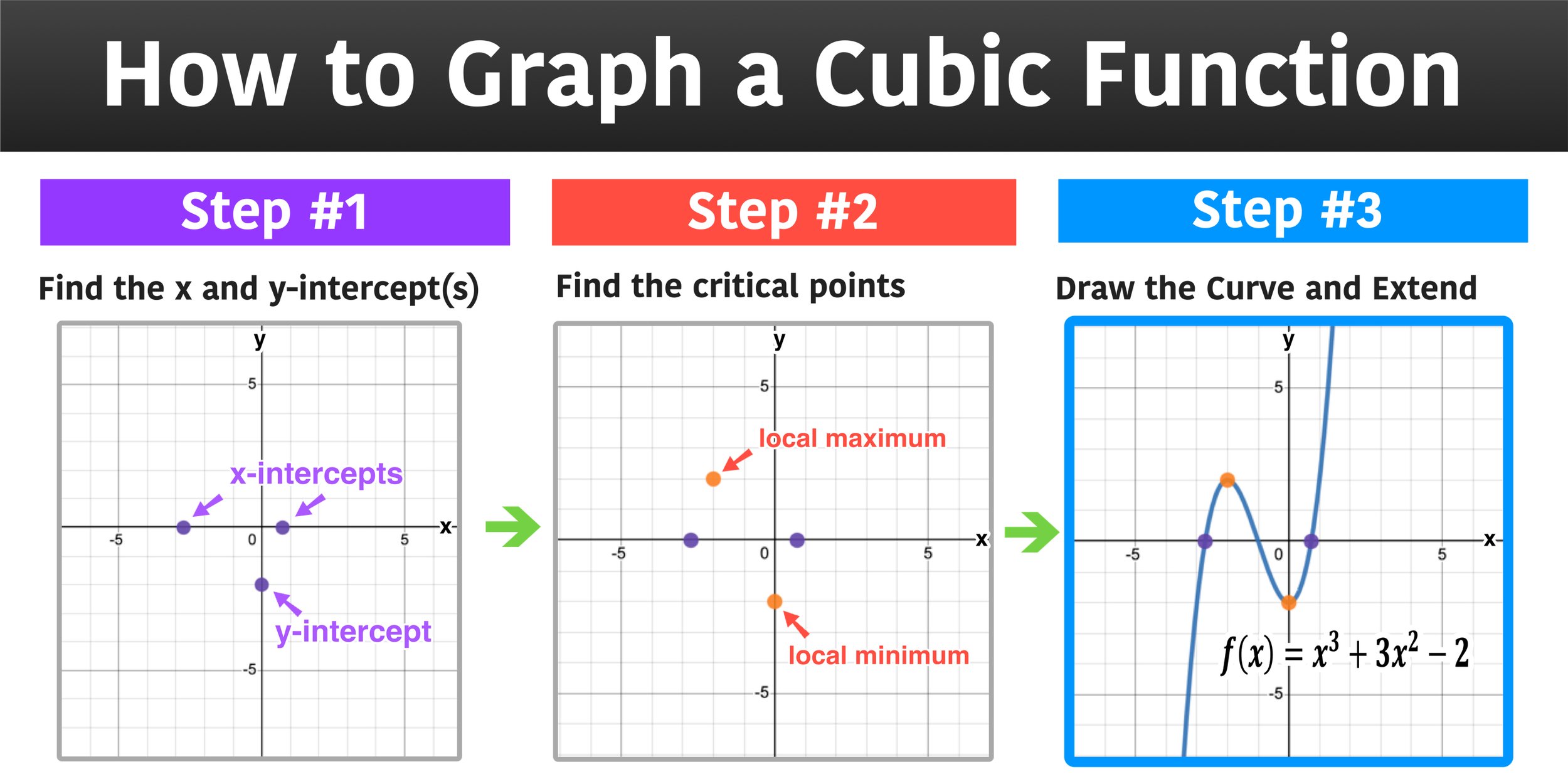
Guide Preview: How to graph a cubic function using 3 easy steps.
Graphing a cubic function is an algebra skill that requires you to draw a graph that represents a 3rd-degree function on the coordinate plane. Unlike graphing a parabola that represents a 2nd-degree function, a cubic function graph has its own unique shape and characteristics.
This complete guide will explore and answer the following:
What does a cubic function graph look like?
How to graph a cubic function in 3 steps
Graphing a cubic function examples
Cubic functions are polynomials that are 3rd-degree functions and appear a lot when studying polynomials. After you’ve learned about graphing linear and quadratic functions, cubic functions are the next obvious step. Graphing a cubic function has similarities to linear and quadratic functions, however, cubic functions have unique characteristics that will be explored in this guide. By the end of this guide, you'll have the skills to graph cubic functions and gain a deeper understanding of their behavior.
Let’s start by comparing the parent graphs of the linear function graph (1st-degree), quadratic function graph (2nd-degree), and cubic-function graph (3rd-degree) as shown in Figure 01 below.
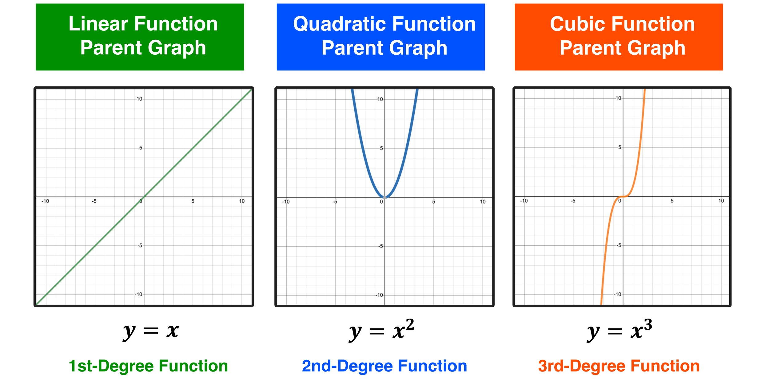
Graphing a Cubic Function: Notice the difference in the shape/behavior of a linear, quadratic, and cubic function graph.
Characteristics of a Cubic Function Graph
Cubic functions are functions of polynomials with the highest degree of 3. A general cubic function can be given as f(x) = ax^3 + bx^2 +cx + d, where a, b,c, and d are arbitrary numbers and a does not equal 0.
The properties that cubic functions share with linear and quadratic functions are:
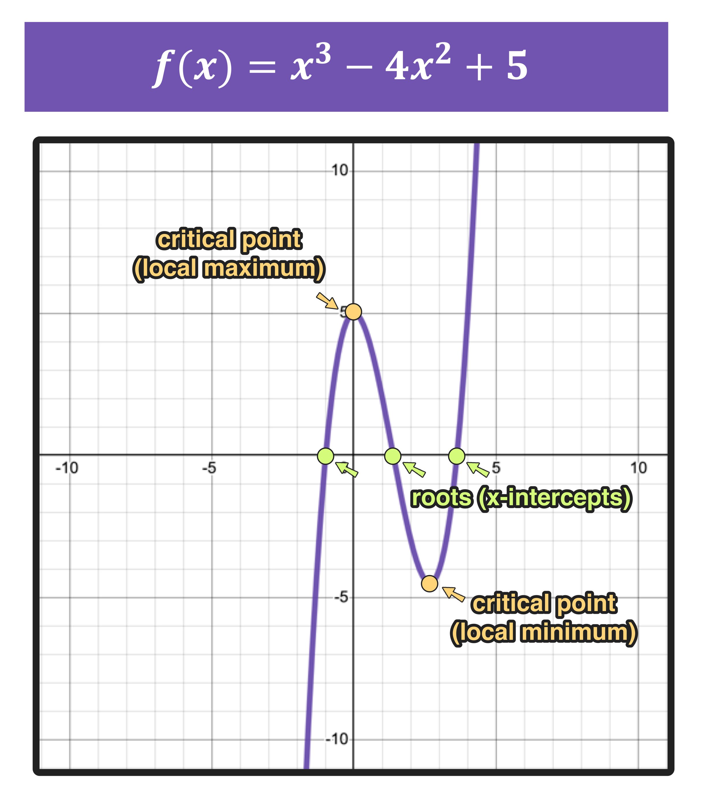
Figure 02: An example of graphing a cubic function with equation f(x)=x^3-4x^2+5. Notice that the function has three roots and two critical points.
The domain is the set of all real numbers
The range is the set of all real numbers
Since both the domain and range span the set of real numbers, there are no vertical or horizontal asymptotes
The maximum number of roots (solutions to f(x) = 0) is the same as the degree of the function. Linear functions have one root, quadratics have a maximum of 2 roots, and 3rd-degree functions, cubic functions, have a maximum of 3 roots.
Some features that distinguish cubic functions from linear and quadratics are:
A cubic function graph has either one or three real roots (x-intercept/s)
A cubic function graph may have two critical points, a local maximum, and a local minimum
A cubic function graph has a single inflection point
Figure 02 shows the end result of graphic a cubic function with equation f(x)=x^3-4x^2+5. Notice that the cubic function graph as three real roots (x-intercepts) and two critical points (a local maximum and a local minimum).
How to Graph a Cubic Function
When graphing a cubic function it is essential to determine the following key features and behaviors of the function.
x and y -intercepts: The x-intercepts, also known as the roots of the function, can be determined by finding the solutions to f(x) = 0. The y-intercept is the value of the function when x = 0, i.e f(0).
Critical points: The local maximum and minimum points, also known as stationary points, are points on the graph where the gradient of the function is 0. To obtain these points, you need to obtain the derivative f’(x) and solve for f’(x) = 0.
Point of inflection: This is the point where the concavity of the curve changes direction. In a cubic function given by f(x) = , the inflection point is given by x=-b/3a
Figure 03 below illustrates examples of critical points and an inflection point on a cubic function graph.
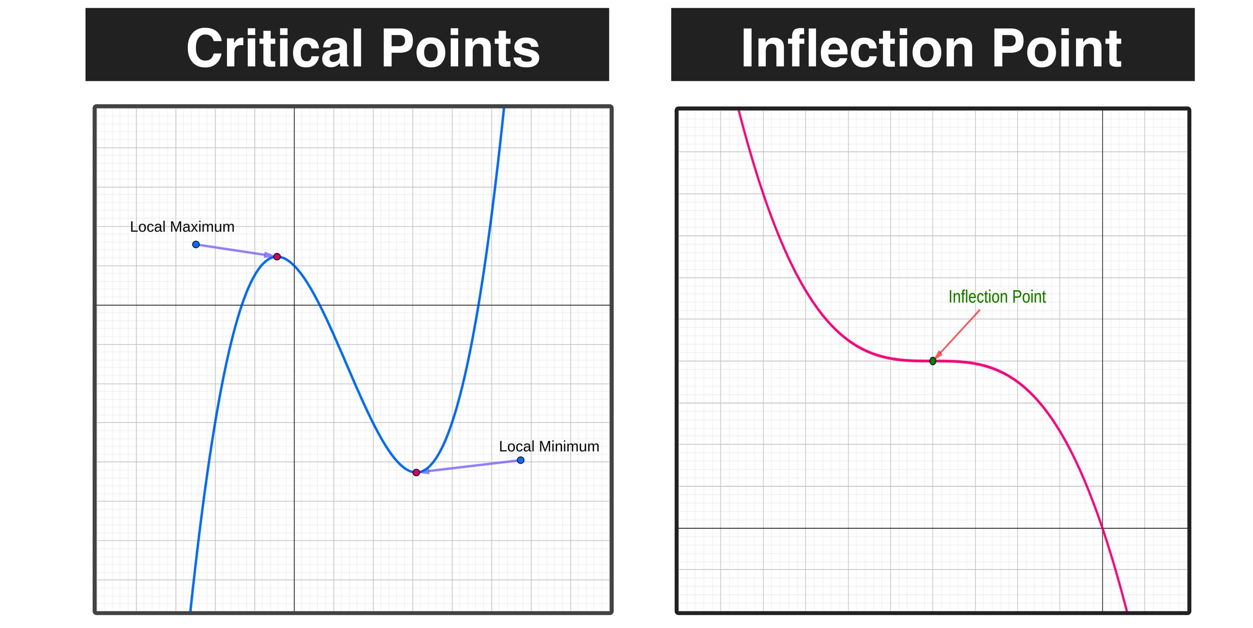
Figure 03: The graph of a cubic function will have two critical points (local maximum and local minimum) and one inflection point, which is the point where the curve of the graph changes direction.
End behaviors: The tendency of the function as x approaches the extremes. With odd-degree polynomials such as cubic functions, the end behaviors can be obtained through the coefficient of the x^3 term.
Figure 04 below shows the end behavior of the graph of a cubic function with a leading coefficient that is positive or negative.
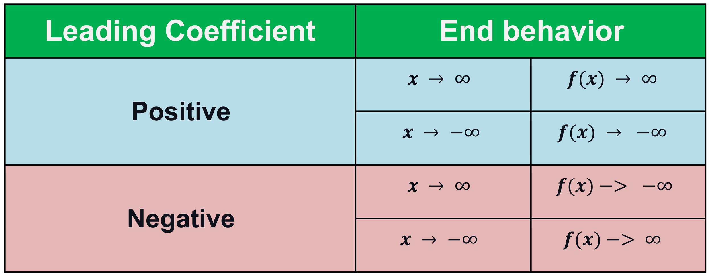
Figure 04: The end behavior of a cubic function graph based on the value and sign of the leading coefficient.
To further visualize the effect of the sign of the leading coefficient on a cubic function graph, take a look at Figure 05 below. Notice the difference in the behavior of the graph when the leading coefficient is a positive value versus when it is a negative value.
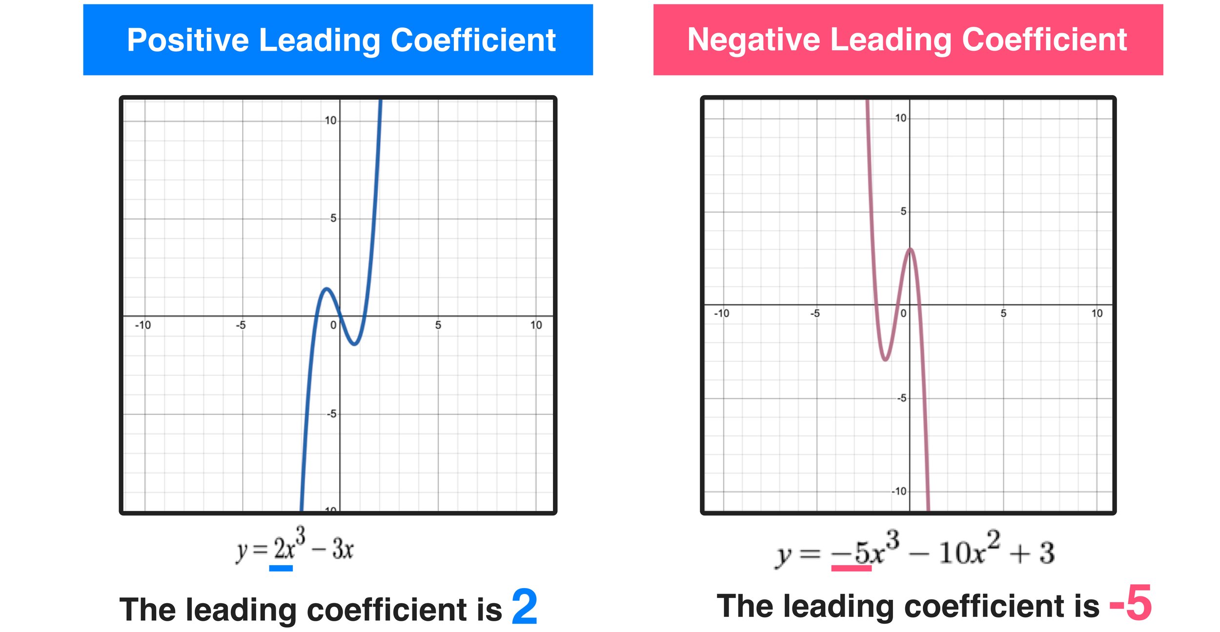
Figure 05: When graphing a cubic function, the sign of the leading coefficient will dictate the end behavior of the cubic function graph and how it will look on the coordinate plane.
Now that you are familiar with the characteristics of the graph of a cubic function, including roots, critical points, the inflection point, and end behavior, let’s take a step-by-step approach to a few examples of graphing a cubic function using a simple 3-step process.
Graphing a Cubic Function Example #1

Figure 06: After completing Step 1 by finding the y-intercept and the x-intercepts, you know that the cubic function graph will pass through the points (0,3), (-3,0), (0.5,0), and (1,0).
Example #1: Graph f(x) = 2x^3 + 3x^2 - 8x +3
To graph a cubic function like the one given in this first example, you can use the following 3-step method:
Step 1: Identify the intercepts
Step 2: Determine the critical points
Step 3: Draw the Curve and Extend
Let’s go ahead and apply these three steps to the given function f(x) = 2x^3 + 3x^2 - 8x +3 as follows:
Step 1: Identify the intercepts
To find the y-intercept, figure out the value of the function when x=0 as follows:
f(0)=2(0)^3 +3(0)^2 - 8(0) + 3 ➝ f(0)= 0 + 0 + 0 + 3 ➝ f(0)= 3
So, the y-intercept of the cubic function is at 3.
To find the x-intercepts, figure out the value of the function when f(x)=0 as follows:
2x^3 + 3x^2 - 8x +3 = 0
It is easier to determine the roots of this cubic function by first factorizing the equation as shown below:
(x-1)(x+3)(2x-1)=0
Now the solutions to the equation become more apparent and can be obtained by equating each factor to 0.
x-1 = 0 ➝ x=1
x+3 = 0 ➝ x=-3
2x -1 = 0 ➝ x=0.5
So, the x-intercepts of the function are at 1, 3, and 0.5.
As shown in Figure 06, after completing Step 1 by finding the y-intercept and the x-intercepts, you know that the cubic function graph will pass through the points (0,3), (-3,0), (0.5,0), and (1,0). Now let’s continue onto the next step.
Step 2: Determine the Critical Points
First, let’s work out the derivative of f(x) by applying the power rule as follows:
f(x) = 2x^3 + 3x^2 - 8x +3
f’(x)= 6x^2 +6x -8
At the stationary points, the derivative (gradient) is 0. Therefore, to obtain the x-coordinates of the stationary points we can equate the derivative f’(x) to 0 by setting f’(x)=0 and solving for x as follows:
6x^2 +6x -8 = 0
You can solve for x by using the quadratic formula: x = [−b ± √(b2 − 4ac)]/2a


Figure 07: After completing Step 2, you now have points plotted at the y-intercept, x-intercepts, and critical points of the cubic function.
By using the quadratic formula, you can conclude that the x-coordinates at the critical points are x≈0.758 and x≈-1.758
Next, let’s substitute the x-coordinates calculated into f(x) and obtain the y-coordinates of the stationary points as follows:
f(0.758) = 2(0.758)^3 + 3(0.758)^2 - 8(0.758) +3 ➝ f(0.758) ≈ -0.469
f(-1.758) = 2(01.758)^3 + 3(-1.758)^2 - 8(-1.758) +3 ➝ f(0.758) ≈ 15.469
Therefore, the critical points are at approximately (0.758 , -0.469) and (-1.758 , 15.469)
As shown in Figure 07, in addition to the y-intercept and x-intercepts of the function, you also have the critical points plotted.
Notably, (0.758 , -0.469) is a local minimum and (-1.758 ,15.469) is a local maximum.
Now you are ready to draw your graph and complete the problem.
Step 3: Draw the Curve and Extend
The final step is to draw a smooth curve that passes across all points.

Before you extend the lines of the graph, it is a good practice to check the end behaviors. Since the leading coefficient (2) of the function is positive the following will be true:

Figure 08: Since the leading coefficient (2) is positive, you know what the end behavior of the cubic function graph will be.
Next, extend the line as needed to cover the relevant domain and range of the function.
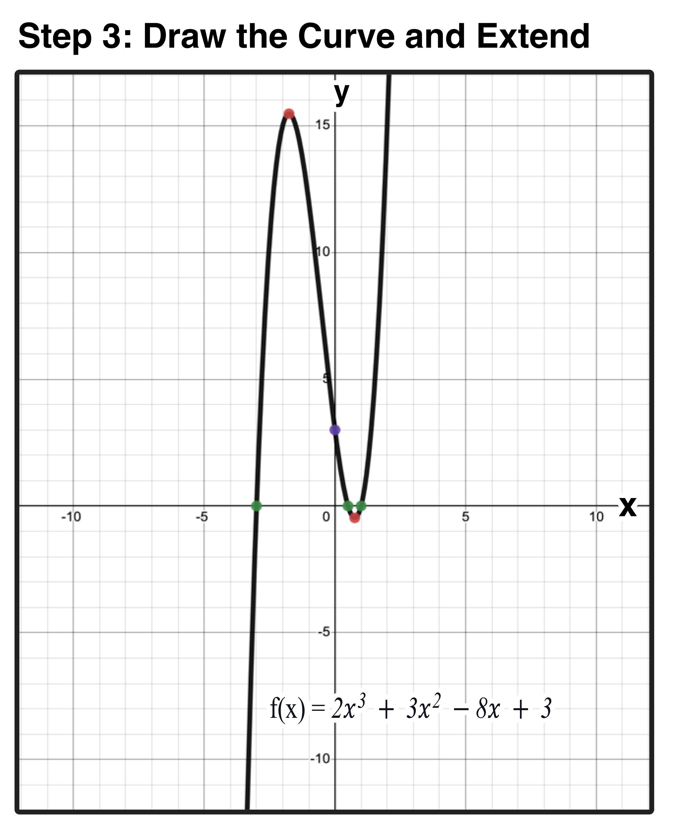
Figure 09: Graphing a Cubic Function: The completed cubic function graph for f(x) = 2x^3 + 3x^2 - 8x +3
You have just completed the cubic function graph for f(x) = 2x^3 + 3x^2 - 8x +3, as shown in Figure 09 above. Before we move onto to working through one more graph a cubic function example, let’s quickly recap how we completed Example #1 using the 3-step method as shown in Figure 10 below.

Figure 10: Visual recap of the 3-step method used to complete the function graph for Example #1.
Graphing a Cubic Function Example #2
Example #2: Graph f(x) = -x^3 + 8
The steps for graphing a cubic function like the one shown in Example #2 are the same three steps that we used in the previous example.

Figure 11: The graph of a cubic function starts with finding and plotting the y and x-intercepts.
Step 1: Identify the intercepts
To find the y-intercept, calculate the value of the function when x=0 as follows:
f(0)= -(0)^3 + 8 ➝ f(0)= 0 + 8 ➝ f(0)= 8
So, the y-intercept of the cubic function is at 8.
To find the x-intercepts, figure out the value of the function when f(x)=0 as follows:
-x^3 + 8 = 0 ➝ x^3 = 8
Hence, the x-intercepts are x = 2, x =-1+√3i , and x = -1-√3i
But, since you are graphing a cubic function on the real plane, you can ignore the two complex roots.
Thus, the graph will contain a single real x-intercept at x = 2.
So, the x-intercept of the function is 2.
As shown in Figure 11, after completing the first step by finding the y-intercept and the x-intercepts, you know that the cubic function graph will pass through the points (0,8) and (2,0).
Step 2: Determine the Critical Points
First, let’s work out the derivative of f(x) by applying the power rule as follows:
f(x) = -x^3 + 8
f’(x)= -3x^2
At the stationary points, the derivative (gradient) is 0. Therefore, to obtain the x-coordinates of the stationary points we can equate the derivative f’(x) to 0 by setting f’(x)=0 and solving for x as follows:
-3x^2 = 0 ➝ x = 0
Next, let’s substitute the x-coordinates calculated into f(x) and obtain the y-coordinates of the stationary points.
f(x) = -x^3 + 8
f(0) = -(0)^3 + 8 ➝ f(0) = 8
Therefore, the stationary point is (0, 8).

Figure 12: Since there is only one stationary point that has the same coordinates of the inflection point, this cubic function graph will not have any local maximum or minimum points.
Next, let’s work out the inflection point of the curve. The x-coordinate of the inflection point is given by
x=-b/3a ➝ x=-0/-3 = 0
The x-value at the inflection point: x=0
The y-coordinate of the inflection point can be obtained by calculating f(0), which you already know is equal to 8.
The y-value at the inflection point: x=8
Therefore, the inflection point is at (0,8).
In this example, the inflection point is identical to the stationary point obtained above. This means that the cubic function f(x) doesn’t have any local maximum or local minimum points but rather a single inflection point at (0,8)
Step 3: Draw the Curve and Extend
Now you are just about ready to construct your cubic function graph. You have already identified two distinct points that the cubic function will pass through (x-intercept and inflection point).
To determine a few additional points that the graph will pass through and improve the accuracy of the curve that you will, you can find several other x and y coordinate pairs. Choose random values of x and calculate the corresponding value of f(x).
For example, to calculate the y-value when x=-1:

Figure 13: Function Table
f(x) = -x^3 + 8
f(-1) = -(-1)^3 + 8 = 9 ➝ f(-1) = 9
Therefore, the graph will pass through the point (-1,9)
You can repeat this process for additional x-values to figure out more points that the cubic function graph will pass through.
The function table shown in Figure 13 includes the three points on the curve that we have already found—(0,8), (2,0), and (-1,9), plus two additional points: (-2,16) and (1,7).
Finally, plot all of the points that you have found and then draw a smooth curve that passes through all of them.
Since the leading coefficient (-1) of the function is negative, remember to follow the end behaviors accordingly.
The graph in Figure 14 below shows the completed graph of the cubic function f(x)=-x^3 + 8.

Figure 14: Graph a Cubic Function Completed
Graphing a Cubic Function: Conclusion
The process to graph a cubic function can be summarized to following the following simple 3-step method:
Identify the y-intercept and the x-intercept(s)
Determining the critical points
Draw the curve and extend
By applying these simple steps, anyone can accurately graph a cubic function and gain insights into its behavior. Mastering the art of graphing cubic functions not only strengthens your understanding of polynomials, but it also provides valuable tools for analyzing real-world situations and making informed decisions.
More Math Resources You Will Love: